Particle Filters

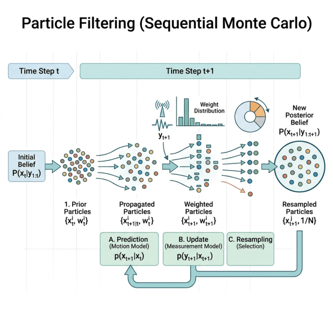
Diagram of sequential Monte Carlo particle filtering steps including prior, propagated, weighted, and resampled particles with prediction, update, and resampling phases
Illustration of the particle filtering algorithm showing prediction, update, and resampling steps.

A particle filter is a method for estimating the hidden state of a system as that system changes over time.

That sounds similar to a Kalman filter, and it is. Both methods are used for filtering. Both methods combine a model of how the system evolves with noisy observations of that system. Both methods are trying to answer the same basic question:

Given everything I have observed so far, what do I believe about the current hidden state?

The difference is how belief is represented.

A Kalman filter represents belief with a Gaussian distribution. In practice, this means it keeps track of a mean and covariance.

A particle filter represents belief with many weighted samples. These samples are called particles.

Each particle is one possible version of the hidden state. The weight attached to that particle tells us how plausible that possible state is.


{xtk, wtk}k=1K


Here, xtk is the k-th particle at time t, wtk is its weight, and K is the total number of particles.

NOTE: A particle is just a sampled hypothesis about the hidden state. A cloud of weighted particles is an approximation to a probability distribution.


What Is a Particle Filter Used For?


Particle filters are used when we need to estimate a hidden state over time, but the uncertainty is too complicated for a simple Gaussian approximation.

They are common in robotics, object tracking, target localization, navigation, nonlinear time-series analysis, ecological modeling, econometrics, signal processing, and fault detection.

A classic example is robot localization.

Suppose a robot is moving through a building. The robot has a map, but it does not know exactly where it is. Its sensors are noisy. Several hallways may look similar. Several locations may explain the same observation.

A particle filter can keep multiple possible robot locations alive at the same time.

  • Some particles may represent the robot being in hallway A.
  • Some particles may represent the robot being in hallway B.
  • Some particles may represent the robot being in a nearby room.

As new observations arrive, the particle filter gives more weight to the particles that better explain the data.

This is the main advantage of particle filters: they do not have to compress uncertainty into one Gaussian blob.


What Problems Are Particle Filters Good For?


Particle filters are useful when uncertainty is complicated.

They are especially good for problems with nonlinear dynamics, nonlinear observations, non-Gaussian noise, ambiguous measurements, multiple possible explanations, tracking under occlusion, sudden changes, or regime switches.

The key idea is that a particle filter can represent a distribution with many shapes.

It can represent skewed uncertainty. It can represent heavy-tailed uncertainty. It can represent uncertainty with several separate modes.

For example, if an object disappears behind another object in a video, there may be several plausible places where it could reappear. A particle filter can keep particles in several of those plausible places until the next observation makes the situation clearer.


A Simple Example: Robot Localization


Suppose a robot is trying to localize itself inside a building.

The hidden state is the robot’s position and orientation.


xt = [x-positiont, y-positiont, orientationt]


The robot receives sensor measurements. These might be distances to walls, visual features from a camera, or laser range measurements.

The observation at time t is:


yt = sensor measurement at time t


At the beginning, the robot may not know where it is. So we initialize many particles across the map.

Each particle is one guess about the robot’s pose.

One particle might say: maybe the robot is in this hallway, facing north.

Another particle might say: maybe the robot is in that room, facing east.

Another particle might say: maybe the robot is near this wall, facing south.

Now the robot moves.

Each particle is moved forward according to the motion model.


xtk ~ p(xt | xt-1k)


This means that the k-th particle at time t is sampled from the transition model, given where that particle was at the previous time step.

In plain language:

Move each possible robot pose forward according to the robot’s motion model, but include motion noise.

Then the robot receives a new sensor measurement.

For each particle, we ask:

If the robot were actually at this particle’s location, how likely would this sensor measurement be?

Particles that explain the measurement well receive high weights. Particles that explain the measurement poorly receive low weights.


wtk ∝ p(yt | xtk)


This says that the weight of particle k is proportional to the likelihood of the observation under that particle.

After computing the weights, we normalize them so they sum to one.


wtk = wtk / Σj=1K wtj


Now the normalized weights can be treated like probabilities over particles.


The Particle Filter Algorithm


The basic particle filter has three main steps.

  1. Propagate the particles through the motion model.
  2. Weight the particles using the new observation.
  3. Resample the particles so that plausible particles survive.

Then repeat.

This is why particle filters are also called Sequential Monte Carlo methods.

“Monte Carlo” means we approximate distributions using samples.

“Sequential” means we update those samples over time as new observations arrive.


Resampling


After a few time steps, many particles may have weights close to zero. Only a few particles may explain the observations well.

This is called particle degeneracy.

Degeneracy means we are wasting computation on particles that no longer matter.

To fix this, particle filters usually resample.

During resampling, high-weight particles are likely to be copied. Low-weight particles are likely to disappear.

Suppose four particles have normalized weights:


[0.05, 0.45, 0.40, 0.10]


The second and third particles are much more likely to survive than the first and fourth particles.

After resampling, we still have the same number of particles, but more of them are concentrated in plausible regions of the state space.

NOTE: Resampling is useful, but it can also reduce diversity. If we keep copying the same high-weight particles, the particle population may lose alternative explanations too quickly.


What Is Required to Set Up a Particle Filter?


To use a particle filter, we need more than just particles. We need to define the probabilistic model that tells the particles how to move, how to compare themselves to data, and how to survive over time.

A particle filter needs five main ingredients.

  1. A hidden state. This is what we are trying to estimate.
  2. A transition model. This tells us how the hidden state evolves from one time step to the next.
  3. An observation model. This tells us how likely an observation is, given a possible hidden state.
  4. An initial particle distribution. This tells us where the particles should start.
  5. A resampling rule. This tells us when and how to copy high-weight particles and remove low-weight particles.

The most important modeling choice is the hidden state.

If the state is too small, the filter will not contain enough information to predict the future. If the state is too large, the filter may need an enormous number of particles to work well.

For a robot, the state might be position and orientation:


xt = [x-positiont, y-positiont, orientationt]


For an object in a video, the state might include position, velocity, width, and height.

For a biological or medical time-series problem, the state might include an unobserved disease burden, a latent response level, or a patient-specific trajectory variable.

The key question is:

What information does the filter need to carry forward so that it can explain future observations?


How to Build the Particle Filter


Once the hidden state is defined, the next step is to define the transition model.

The transition model answers:

If the system is currently in this state, where could it plausibly go next?

In notation, we write this as:


xt ~ p(xt | xt-1)


This means the next state is sampled from a distribution that depends on the previous state.

For a robot, this might use a motion model. If the robot moves forward, each particle moves forward too, but with some noise. That noise matters because real movement is imperfect.

After defining the transition model, we define the observation model.

The observation model answers:

If this particle were the true state, how likely would the observed data be?

This is the likelihood:


wtk ∝ p(yt | xtk)


This is where the data enters the filter. A particle survives because it predicts observations that look like the observations we actually received.

Then we normalize the weights, resample particles, and repeat the process at the next time step.

In practice, the workflow looks like this:

  1. Choose the hidden state.
  2. Initialize many particles.
  3. Move each particle forward using the transition model.
  4. Compare each particle to the new observation.
  5. Assign a weight to each particle.
  6. Normalize the weights.
  7. Resample if the particle population has degenerated.
  8. Use the resulting particles to estimate the current state.

For example, the current state estimate might be the weighted average of the particles, but that is not always the only useful summary. Sometimes the full particle cloud is more informative than a single average.

NOTE: If the posterior has two modes, the weighted average may fall between them and may not represent a realistic state. In that case, it is better to inspect the particle distribution itself.


What to Look For


When a particle filter is working well, the particles should behave in a sensible way.

Early on, the particles may be spread out because uncertainty is high. As observations arrive, particles should begin concentrating in regions that explain the data well.

Good signs include:

  • particles concentrate around plausible states,
  • high-weight particles are consistent with observations,
  • the filter does not collapse too early,
  • multiple hypotheses survive when the data are genuinely ambiguous,
  • uncertainty decreases when observations are informative,
  • uncertainty increases when observations are missing or noisy.

The particle cloud should tell a story. If the data are clear, the particles should agree. If the data are ambiguous, the particles should preserve that ambiguity instead of pretending to be certain.


What to Watch Out For


Particle filters are flexible, but they can fail in predictable ways.

The first problem is particle degeneracy.

This happens when almost all particles have tiny weights and only a few particles carry most of the probability mass.

A common diagnostic is the effective sample size. It estimates how many particles are actually contributing.


ESS = 1 / Σk=1K (wtk)2


If the effective sample size is low, the filter is relying on too few particles. That usually means resampling is needed.

The second problem is particle impoverishment.

This happens after resampling, when many particles become copies of the same high-weight particles. The filter may look confident, but it has lost diversity.

This can be dangerous because the filter may commit too early to one explanation and lose other plausible hypotheses.

The third problem is a poor transition model.

If the transition model does not allow particles to move into the region where the true state is, then the filter cannot recover. No amount of weighting can save particles that never reach plausible states.

The fourth problem is a poor observation model.

If the likelihood is too sharp, the filter may kill off too many particles. If the likelihood is too broad, the observations may not influence the particles enough.

The fifth problem is too few particles.

Particle filters can struggle in high-dimensional spaces because the number of particles needed may grow very quickly. This is one reason particle filters are powerful but not magical.

In practice, you should watch for these warning signs:

  • one particle receives almost all the weight,
  • particles collapse into a tiny region too early,
  • particles remain spread out even after informative observations,
  • the filter is very sensitive to random seed,
  • state estimates jump erratically,
  • the weighted average gives an impossible or meaningless state.

When these happen, the issue is usually not just the particle filter algorithm. It is often the model setup: the state definition, transition model, observation model, noise assumptions, or number of particles.


A Practical Way to Think About It


A particle filter is not just a computational trick. It is a way of carrying uncertainty through time.

To set it up well, think like this:

What are the possible states of the world?

How can those states evolve?

What observations would each state produce?

Which possible states should survive after seeing the data?

That is the whole logic of the particle filter.

The particles represent possible states. The transition model moves them forward. The observation model scores them. Resampling reallocates computation toward the states that remain plausible.

If those pieces are well designed, the filter can represent complicated uncertainty in a way that a single Gaussian belief cannot.


The Bayesian View


The goal of filtering is to estimate:


p(xt | y1, …, yt)


This is the distribution of the current hidden state, given all observations so far.

A Kalman filter solves this exactly when the model is linear and Gaussian.

A particle filter approximates this distribution using weighted particles.


p(xt | y1, …, yt) ≈ Σk=1K wtk δ(xt − xtk)


This notation says that the posterior distribution is approximated by point masses at the particles, weighted by their normalized weights.

The symbol δ represents a point mass. In plain language, it places probability directly on a particle.

You do not need to love this notation to understand the idea.

The posterior is represented by many weighted guesses instead of by one Gaussian distribution.


Discussion


Particle filters are powerful because they can keep multiple hypotheses alive.

This matters when observations are ambiguous.

Suppose a robot could be in two similar-looking rooms. A Kalman filter may average those two possible locations and place the robot somewhere between them. A particle filter can place some particles in one room and some particles in the other room.

Then, as more observations arrive, the particles in the better location receive higher weights and survive.

So the particle filter does not have to decide too early.

That flexibility is the main advantage.

But flexibility has a cost.

Particle filters can be computationally expensive. If the state space is high-dimensional, we may need many particles to approximate the posterior well.

If we use too few particles, the filter can collapse onto a small number of states. Resampling helps with degeneracy, but it can also reduce diversity.

So particle filters are not automatically better than Kalman filters.

A Kalman filter is usually better when the system is approximately linear, Gaussian, and real-time efficiency matters.

A particle filter is usually better when the posterior is nonlinear, non-Gaussian, multimodal, or ambiguous.

The simplest summary is:

A Kalman filter tracks one Gaussian belief over time.

A particle filter tracks many possible states over time.

Both are Bayesian filters.

They differ mainly in how they represent uncertainty.
Kalman Filter

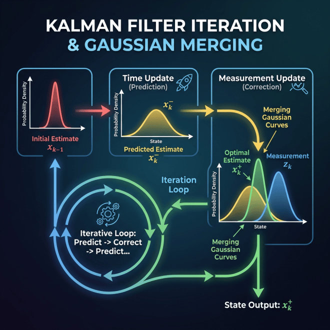
Flowchart showing Kalman filter iteration with time update, measurement update, and merging Gaussian curves
Diagram illustrating the iterative Kalman filter steps including time update, measurement update, and Gaussian curve merging.

A Kalman filter is a method for estimating the hidden state of a system as that system changes over time.

That sounds abstract, so let’s make it concrete.

Suppose we are tracking something that moves: a drone, a robot, a car, a satellite, or even a signal in a sensor. The object has a true state, but we do not get to observe that state perfectly.

For example, a drone has a true position and velocity. But our sensor may only give us a noisy measurement of position.

So we have two things:

1. The real state of the system.

2. A noisy observation of that state.

The job of the Kalman filter is to combine these two pieces of information over time.

It asks:

Given what I believed before, and given the noisy measurement I just received, what should I believe now?

This is the basic filtering problem.

What Is a Kalman Filter Used For?

Kalman filters are used for real-time state estimation.

They are common in navigation, robotics, aerospace engineering, control systems, computer vision, economics, and signal processing.

A classic example is GPS tracking.

GPS measurements are noisy. If you look at raw GPS data, the estimated position may jump around even when the object is moving smoothly. A Kalman filter can smooth those measurements by combining them with a motion model.

The motion model says something like:

If the object was here before, and it was moving with this velocity, then it should probably be over here now.

The measurement says:

The sensor thinks the object is here.

The Kalman filter combines both.

It does not blindly trust the model.
It does not blindly trust the sensor.
It balances them according to their uncertainty.

What Problems Are Kalman Filters Good For?

Kalman filters are especially good for problems where the system is approximately linear and the noise is approximately Gaussian.

In simple terms, this means:

  • the system evolves in a fairly smooth way,
  • measurements are noisy but not wildly unpredictable,
  • uncertainty can be reasonably represented by a bell-shaped distribution.

The Kalman filter represents belief using two things:

  • a mean,
  • a covariance.

The mean is the best estimate of the hidden state.

The covariance describes how uncertain we are about that estimate.

So instead of storing every possible state the system could be in, the Kalman filter stores a compact summary of belief.

That is why it is so efficient.

A Simple Example

Suppose we are tracking a drone moving in one dimension.

The hidden state contains position and velocity.

xt=[positiont,velocityt]x_t = [position_t, velocity_t]

The sensor only measures position, and the measurement is noisy.

yt=noisy position measurementy_t = \text{noisy position measurement}

At time t-1, suppose the drone is estimated to be at position 10 and moving with velocity 2.

Before seeing the next measurement, the model predicts that the drone should be near position 12.

That is the prediction step.

Then the sensor reports position 13.5.

Now we have a disagreement.

The model says: I expected the drone near 12.

The sensor says: I measured the drone near 13.5.

The Kalman filter combines these two pieces of information.

If the sensor is very reliable, the updated estimate moves closer to 13.5.

If the sensor is noisy, the updated estimate stays closer to 12.

This balance is controlled by the Kalman gain.

The Kalman gain determines how much the filter trusts the new measurement compared to the model prediction.

The Model

A standard Kalman filter assumes a linear state-space model.

The state evolves like this:

xt=Axt−1+errorx_t = A x_{t-1} + error

The observation is generated like this:

yt=Cxt+errory_t = C x_t + error

The first equation says that the current state depends on the previous state.

The second equation says that the observation is a noisy measurement of the current state.

Here, A describes the system dynamics. For example, it tells us how position and velocity change over time.

The matrix C describes what part of the hidden state we actually observe.

NOTE: We may care about both position and velocity, but only measure position directly. The velocity still matters because it helps predict future position.

The Bayesian View

The Kalman filter is a Bayesian filter.

That means it keeps updating a probability distribution over the hidden state as new observations arrive.

The object we want is the filtering distribution:

p(xt|y1,…,yt)p(x_t | y_1, …, y_t)

This means: the probability distribution of the current hidden state, given all observations so far.

The Kalman filter is special because, under linear Gaussian assumptions, this distribution stays Gaussian.

So the filter does not need to store a complicated distribution.

It only stores the mean and covariance.

That is the entire reason the Kalman filter is so clean.

Discussion

The Kalman filter is powerful because it is fast, elegant, and interpretable.

It is fast because it only updates a mean and covariance.

It is elegant because it gives the exact Bayesian filtering solution when the model is linear and Gaussian.

It is interpretable because the uncertainty has a clear meaning. If the covariance is large, the filter is uncertain. If the covariance is small, the filter is confident.

But the Kalman filter also has limitations.

The main limitation is that it represents uncertainty as one Gaussian distribution.

That is fine when the uncertainty has one main center.

But suppose a robot is in a building and there are two hallways that look almost identical. The robot may plausibly be in hallway A or hallway B.

That belief has two modes.

A Kalman filter may average those two possibilities and put the robot somewhere between the hallways, possibly inside a wall.

That is not just a bad estimate. It is a bad representation of uncertainty.

So the Kalman filter works best when one Gaussian belief is a reasonable approximation.

When the posterior distribution is nonlinear, non-Gaussian, or multimodal, we often need something more flexible.

That leads us to particle filters.

How to Think Through a Kalman Filter Problem

When setting up a Kalman filter, the hardest part is usually not the algebra. The hardest part is deciding what the hidden state should be and how the measurements relate to that state.

A good way to think through the problem is to ask four questions.

First:

What am I trying to estimate?

This determines the hidden state (xtx_t).

For the drone example, we may want to estimate both position and velocity:

xt=[positiont velocityt]x_t = \begin{bmatrix} \text{position}_t \ \text{velocity}_t \end{bmatrix}

Even if we only measure position, velocity is still useful because it helps us predict future position.

Second:

How does the state evolve from one time step to the next?

This determines the transition model.

For a simple constant-velocity model, position changes according to velocity. If the time step is (Δt\Delta t), then:

positiont=positiont−1+Δt⋅velocityt−1\text{position} t = \text{position}{t-1} + \Delta t \cdot \text{velocity}_{t-1}

and velocity may stay approximately the same:

velocityt=velocityt−1\text{velocity}t = \text{velocity}{t-1}

In matrix form, this becomes:

xt=Axt−1+ϵtx_t = A x_{t-1} + \epsilon_t

where (A) is the state-transition matrix and (ϵt\epsilon_t) is process noise.

For this constant-velocity example, the transition matrix is:

A=[1amp;Δt 0amp;1]A = \begin{bmatrix} 1 & \Delta t \ 0 & 1 \end{bmatrix}

This matrix says:

  • new position equals old position plus velocity times time,
  • new velocity equals old velocity.

Third:

What do I actually observe?

This determines the observation model.

If the sensor only measures position, then the observation is:

yt=noisy position measurementy_t = \text{noisy position measurement}

In matrix form:

yt=Cxt+δty_t = C x_t + \delta_t

where (C) selects the part of the hidden state that the sensor can observe.

For position-only measurements,

C=[1amp;0]C = \begin{bmatrix} 1 & 0 \end{bmatrix}

This means:

observe position, but do not directly observe velocity.

Fourth:

How noisy are the model and the measurements?

This determines the covariance matrices.

The process-noise covariance (Q) describes uncertainty in the dynamics. It answers:

How much do I trust my motion model?

The measurement-noise covariance (R) describes uncertainty in the sensor. It answers:

How much do I trust my observations?

If (R) is large, the measurements are noisy, so the filter trusts the model more.

If (R) is small, the measurements are reliable, so the filter trusts the observations more.

If (Q) is large, the model dynamics are uncertain, so the filter is more willing to adjust when new measurements arrive.

If (Q) is small, the model is trusted more strongly.

NOTE: Choosing (Q) and (R) is one of the most important practical parts of using a Kalman filter. The equations may be correct, but poor noise assumptions can make the filter behave badly.

What Is Required?

To run a Kalman filter, we need five main ingredients.

  1. An initial state estimate.
μ0\mu_0

This is our best guess of the starting state.

  1. An initial uncertainty estimate.
Σ0\Sigma_0

This says how uncertain we are about the initial state.

  1. A transition model.
AA

This describes how the state evolves.

  1. An observation model.
CC

This describes how the hidden state produces measurements.

  1. Noise covariances.
QandRQ \quad \text{and} \quad R

The matrix (Q) describes process noise.
The matrix (R) describes measurement noise.

Once these are specified, the Kalman filter can run recursively.

How the Solution Proceeds

At each time step, the Kalman filter performs two operations: prediction and update.

The prediction step asks:

Before seeing the new measurement, where do I expect the state to be?

The predicted mean is:

μt|t−1=Aμt−1\mu_{t|t-1} = A\mu_{t-1}

The predicted covariance is:

Σt|t−1=AΣt−1AT+Q\Sigma_{t|t-1} = A\Sigma_{t-1}A^T + Q

The update step asks:

After seeing the new measurement, how should I revise my belief?

First, compute the innovation:

rt=yt−Cμt|t−1r_t = y_t – C\mu_{t|t-1}

The innovation is the difference between what we observed and what the model expected us to observe.

Then compute the innovation covariance:

St=CΣt|t−1CT+RS_t = C\Sigma_{t|t-1}C^T + R

This describes how uncertain we are about the innovation.

Then compute the Kalman gain:

Kt=Σt|t−1CTSt−1K_t = \Sigma_{t|t-1}C^T S_t^{-1}

The Kalman gain determines how strongly the new measurement should change the estimate.

Finally, update the mean and covariance:

μt=μt|t−1+Ktrt\mu_t = \mu_{t|t-1} + K_t r_t
Σt=(I−KtC)Σt|t−1\Sigma_t = (I – K_t C)\Sigma_{t|t-1}

Then the filter moves to the next time step and repeats the same process.

The Practical Recipe

So the practical recipe is:

  1. Define the hidden state.
  2. Define how the state evolves.
  3. Define what the sensor observes.
  4. Estimate the process noise (Q).
  5. Estimate the measurement noise (R).
  6. Initialize the state mean and covariance.
  7. Repeat prediction and update as new measurements arrive.

This is why the Kalman filter is so useful.

Once the problem is written as a state-space model, the filtering procedure is automatic.

The real modeling work is deciding what belongs in the state, how the state evolves, what the observations measure, and how much uncertainty belongs in the model and the sensor.

Just got certified as an MLExpert!

MLExpert @ AlgoExpert Issued Mar 2023 Credential ID d747fd0242

What did I have to do?
1. Go through all the courses
2. Solve 10 ML programming questions
2. Take a 75 question quiz under 45 minutes and score above an 80% – I got a 96!

(1/2) ML COURSES

Supervised Learning:
1. Naive Bayes
2. Performance
3. Naive Bayes Optimization
4. K Nearest Neighbors
5. Decision Trees
6. Linear Regression
7. Logistic Regression
8. Support Vector Machine

Unsupervised Learning
1. K-means
2. Singular Value Decomposition

Deep Learning
1. Neural Networks
2. Convolutional Neural Networks
3. Recurrent Neural Networks
4. Generative Adversarial Networks

Recommender Systems
1. Collaborative and Content Based Filtering

Ranking
1. Learning to Rank

(2/2) Large-scale ML

Data Support
1. Data Ingestion
2. Data Storage
3. Data Processing
4. Process Orchestration

Exporation
1. Workspaces

Experimentation
1. Frequentist AB Testing
2. Bayesian AB Testing
3. Multi-Armed Bandit
4. Impact Estimation

Large-Scale Training
1. Basic Models
2. Deep Learning Models
3. Model Validation

Productionization
1. Productionization

Hosting
1. Data Hosting
2. Model Hosting


Sequential Monte Carlo (SMC)

We begin with a short recap of all the previous algorithms we discussed that are prerequisite to Sequential Monte Carlo. Then I intuitively describe how SMC works. After, we dig into the math behind SMC. We first discuss how importance weights are calculated at each time step, and then we discuss how SMC maintains this notion of survival of the fittest with sample trajectories through resampling.

Before we start, I’d like to thank Jan-Willem van de Meent for his lectures in his Advance Machine Learning Class for PhD students at Northeastern University. The images shown are inspired by his lectures. In addition, I’d like to address that more details on SMC can be found in An Introduction to Probabilistic Programming available [arXiv]. This book is intended as a graduate-level introduction to probabilistic programming languages and methods for inference in probabilistic programs.

Mini Review

Before we move on to other Monte Carlo estimators we might use in machine learning, let’s recap:

  • We have discussed what a Monte Carlo Estimator is. It helps us estimate an expectation of some function via sampling.
  • We introduce Importance Sampling as our first Monte Carlo Estimator. We learn that Importance Sampling requires us to evaluate samples using a normalized density, which is something we cannot do (almost always).
  • Then we describe Self-Normalized Importance Sampling (SNIS). SNIS uses two Monte Carlo Estimators; the same one in Importance Sampling and a second one to estimate the normalization constant. This allows us to evaluate samples via an unnormalized density, which we have access to.
  • Importance Sampling methods give us marginal likelihoods, but the downfall is that they do random guessing.
  • We then discuss Monte Carlo Markov Chains (MCMC). MCMC uses transition kernels that let us stay in the target density once we have a good sample (one from the target density). However, (almost always) successful MCMC algorithms need to satisfy detailed balance.
  • We learn that Metropolis-Hastings (a fancy MCMC algorithm) let’s us use any proposal due to an acceptance probability it uses to manage detailed balance for us.
  • In the previous post, we describe an algorithm that marries Importance Sampling and MCMC, Annealing Importance Sampling. This algorithm successfully breaks a hard problem into a series of simpler problems. It provides a marginal likelihood and uses a transition kernel.

Now we will introduce another Monte Carlo Estimator that is used for a set of different problems in machine learning, Sequential Monte Carlo.

Tick Tock: Introducing Time to the Problem!

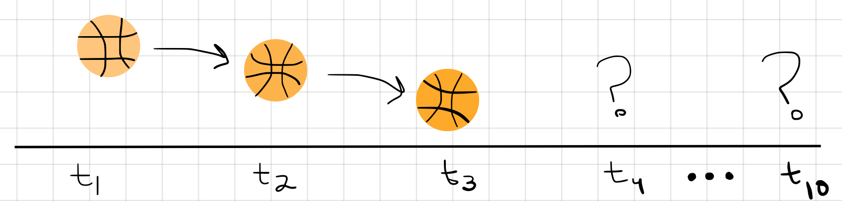
All of the algorithms we have discuss so far are for problems for which we do not need to consider the element of time! What does that mean? Let’s consider an example of looking at a sequence of video frames of a basketball moving from time frame to time frame.

We record that at time t_1 (which can be any arbitrary time stamp), the ball to be up high. We continue to watch the ball move at t_2 and t_3, steadily moving downward. The question we have is, “Where will the ball be in the future? This time-dependent data is referred to as time-series data.
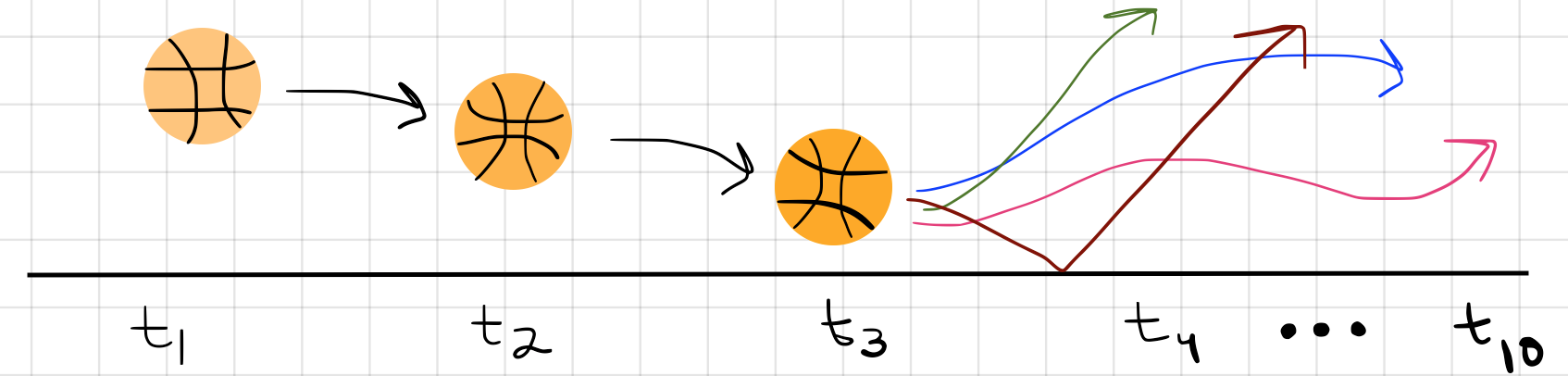
There are many combinations of future movements the ball can make. Several can make sense by following the laws of physics, others can be absolutely garbage (like the ball suddenly shooting upwards, or spelling out a word).

Now consider using any of the Monte Carlo Estimating algorithms we have already discussed. If our data is time dependent, then Importance Sampling would have a very difficult time picking up a pattern that correlates movements between frames. It would probably take ages to get a good set of samples from the posterior! Instead, we can use a more appropriate algorithm for time-dependent problems, such as Sequential Monte Carlo (SMC).

Intuition behind Sequential Monte Carlo

SAMPLING BUDGET. Let’s start off by stating that every sampling scheme has this notion of a sampling budget. This sampling budget (or sample budget) is the maximum number of samples we can afford to use. The number in our budget may depend on the computer we use, the dimensionality of the problem, or even just the amount of time we can afford running our algorithm (because these algorithms do take time!). Usually we use the notation S to represent the number of samples in our sample budget, x^1, x^2, ... x^S.

In time-series problems, we perform inference (using some form of Monte Carlo Estimator) at each time step. This means we use the same number of samples for each time step, i.e. the number of samples in our sampling budget, S.

NOTE: People have adopted the term particle to replace the term sample. Instead of saying we have a sampling budget of 10 samples… it’s common to say we have a sampling budget of 10 particles.

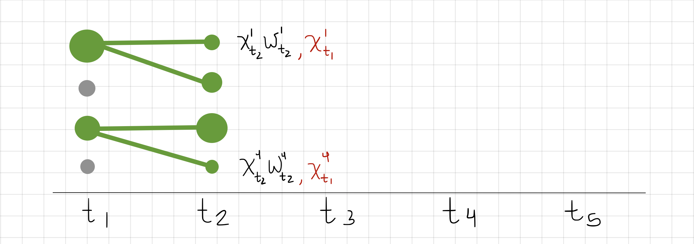
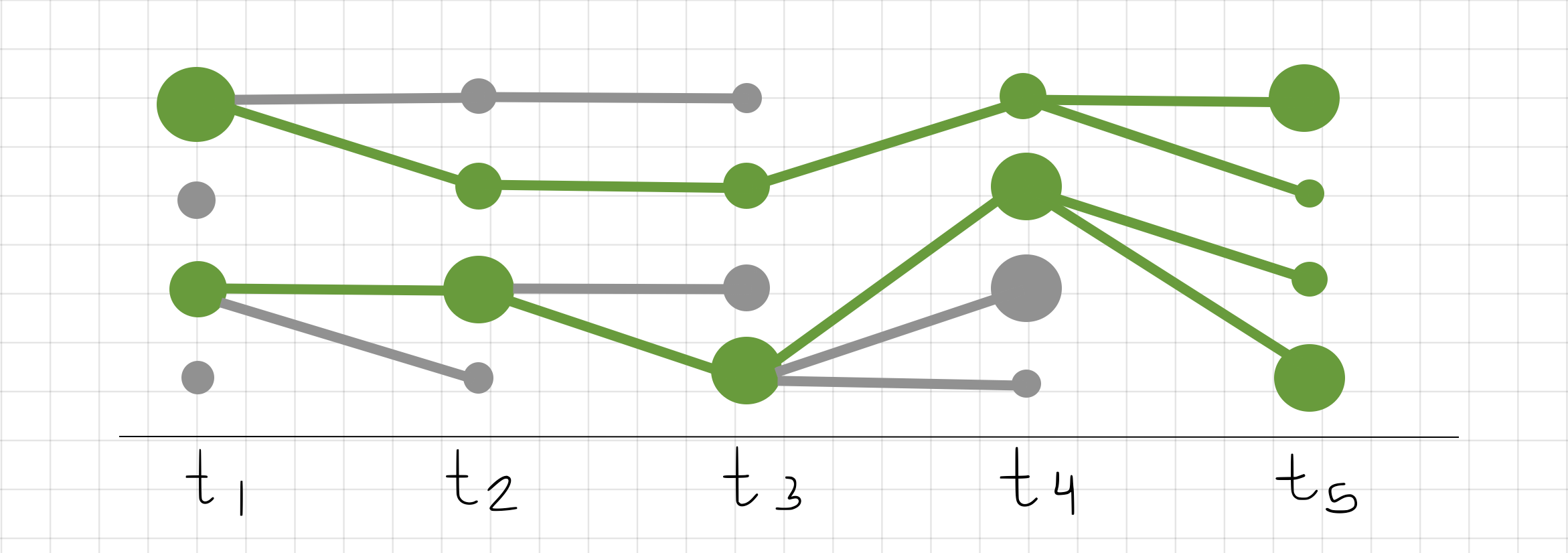
So let’s now consider an example where we have a sampling budget of four, S= 4, and we are working with a small problem with five time steps, t_1, ... t_5. Imagine that each sample represents the position of the ball at its respective time frame. Below we show an example where we have 4 samples at t_1, represented by circles, x^1, x^2, ..., x^4. You can image that these samples represent 4 guesses of the position of the ball for the data from the video frame. Now imagine that each sample (or ball position) has an associated importance weight (just like we discussed in Importance Sampling), (x^1, w^1), (x^2, w^2), ..., (x^4, w^4). The weight tells us how well the ball position matches the data in the video frame. In the figure below, I drew larger circles to represent higher importance weights and smaller circles to represent lower importance weights.
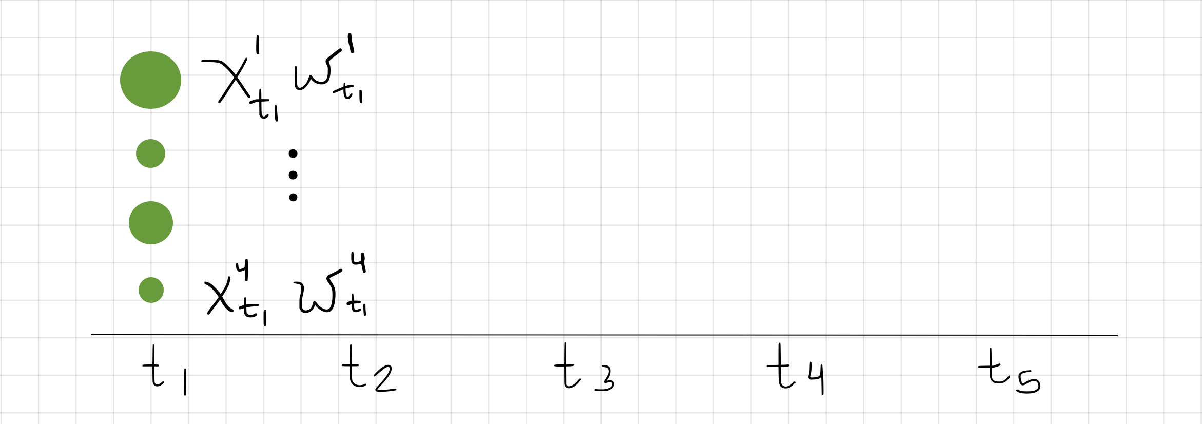
So what SMC does next is decide which samples we should keep and which ones which throw away. This is a way of saying that some guesses of the ball’s position are going to be good ones, and some will be not so good. We want to keep working with our already good guesses at the next time step, so that we can build on those guesses with other guesses. We do this by resampling. This means we will sample with replacement 4 new samples to build on in the next time step, t_2. We resample based by their weights (we’ll go more into detail in a bit).

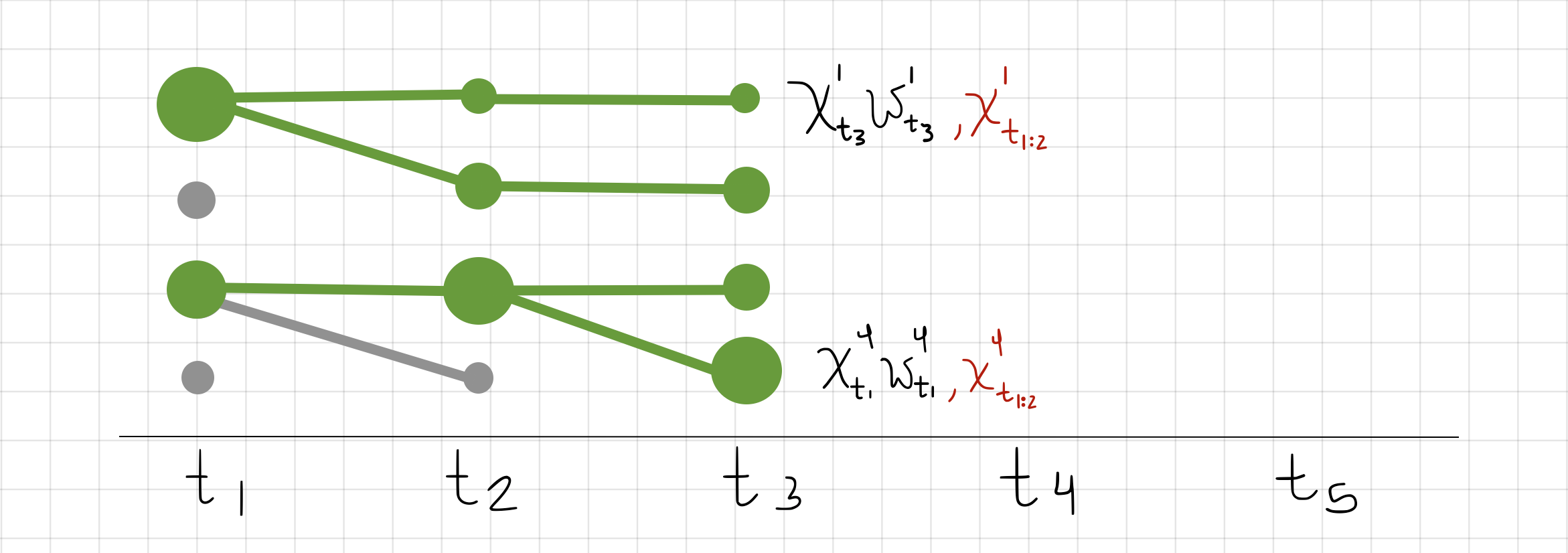
In the figure above, it so happened that we resampled x^1_{t_1} twice and x^3_{t_1} again, twice. This means that those samples for the ball’s position were really good, and we want to keep working with those samples. Now at t_2, we sample new ball positions for that time step, (x^s_{t_2}, w^s_{t_2}), but keep into account the ball positions we resampled from the past (red notation above, x^{s}_{t_1}).

If we move on to t_3, we start to notice how certain trajectories (such as the one in gray) start dying out. This means that some sequences of ball positions will NOT be used for at future time steps.

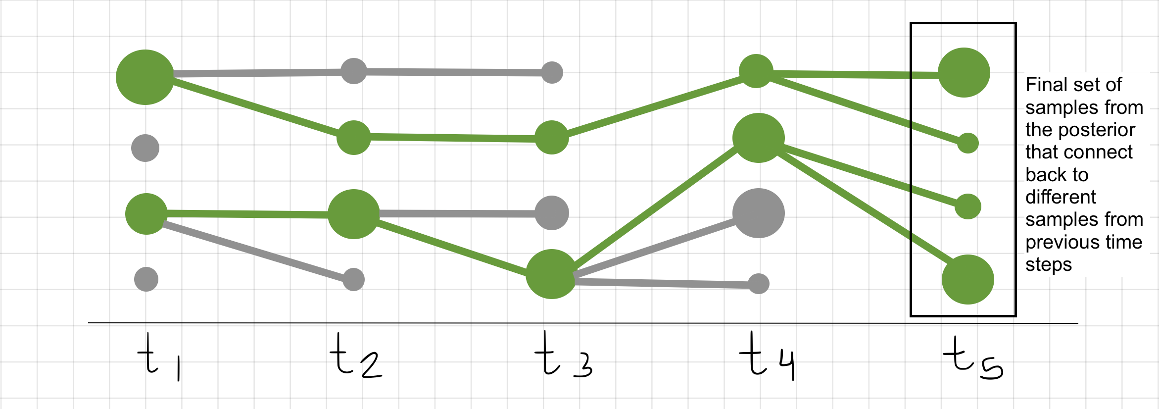
We can continue this pattern until we reach the last time step, t_5. We will see that by then we still have 4 samples. However these 4 samples represent full trajectories, x^{1}_{t=1:5}, ... , x^4_{t=1:5}; these samples connect back to previous time steps. Full trajectories represent entire sequences of ball movements. The ones that survived are the ones that best match our video frame data.

Now that we have described how SMC behaves, let’s be a bit more precise and dig into the math. Don’t worry, I’ll explain it as I use it.

Math Behind Sequential Monte Carlo

Let’s break this discussion into 2 parts. We’ll first discuss the Importance Sampling bit of SMC, and then we’ll discuss Importance Resampling.

Idea 1: Sequential Importance Sampling

As we previously mentioned, our samples have an associated importance weight. In a Monte Carlo estimate, an importance weight of a sample is evaluated in the same pattern we have seen before, with some unnormalized density and the proposal, w =\frac{\gamma(x)}{q(x)}.

Since we are now working with time-series data, we are working with a sequence of samples. Remember that with any problem we have data we observe, y, and data we are trying to learn, x (sometimes referred to as states, or hypothesis). In the example above, y would be the video frame data and x would be the positions of the ball that we are trying to learn/predict.

So in Sequential Monte Carlo, our importance weight really looks more like this:

w_t = \frac{p(y_{1:t}, x_{1:t})}{q(x_{1:t})}

where p(y_{1:t}, x_{1:t}) represents our unnormalized density and q(x_{1:t}) is our proposal. These two distributions take time into consideration; meaning that the densities account for all the samples at each time step.

NOTE: p(y_{1:t}, x_{1:t}) is equivalent to p(y_1, y_2, ...., y_t, x_1, x_2, ..., x_t)

Let’s expand our unnormalized density using the chain rule:

p(y_{1:t}, x_{1:t}) = p(y_{t}, x_{t} \mid x_{1:t-1}) p(y_{1:t-1}, x_{1:t-1})

This is a way of expressing the density that predicts the t^{th} video frame and ball position given the previous 1 : (t-1) video frames and ball positions.

And let’s do the same for our proposal distribution:

q(x_{1:t}) = q(x_{t} \mid x_{1:t-1}) q(x_{1:t-1})

Now that we have these two expanded forms of the distribution, let’s see how they look as an importance weight.

w = \frac {p(y_{t}, x_{t} \mid x_{1:t-1}) } { q(x_{t} \mid x_{1:t-1})} \frac{p(y_{1:t-1}, x_{1:t-1})}{ q(x_{1:t-1})}

This looks kind of messy. Let’s clean it up a bit. Remember that using chain rule, we could expand our unnormalized density as p(y_{1:t}, x_{1:t}) = p(y_{t}, x_{t} \mid x_{1:t-1}) p(y_{1:t-1}, x_{1:t-1}). Notice how we can solve for p(y_{t}, x_{t} \mid x_{1:t-1}):

p(y_t, x_t|x_{1:t-1}) = \frac{p(y_{1:t}, x_{1:t})}{p(y_{1:t-1}, x_{1:t-1})}

If we replace p(y_t, x_t|x_{1:t-1}) in the importance weight with the fraction above:

w_t = \frac {p(y_{1:t}, x_{1:t}) } { p(y_{1:t-1}, x_{1:t-1}) q(x_{t} \mid x_{1:t-1})} \frac{p(y_{1:t-1}, x_{1:t-1})}{ q(x_{1:t-1})}

we can recognized that the second fraction is an importance weight for the previous time step:

w_{t-1} = \frac{p(y_{1:t-1}, x_{1:t-1})}{ q(x_{1:t-1})}

which means our sequential importance weights are updated from time step to time step based on previous weights:

w_t = \frac {p(y_{1:t}, x_{1:t}) } { p(y_{1:t-1}, x_{1:t-1}) q(x_{t} \mid x_{1:t-1})} \frac{p(y_{1:t-1}, x_{1:t-1})}{ q(x_{1:t-1})}
= \frac {p(y_{1:t}, x_{1:t}) } { p(y_{1:t-1}, x_{1:t-1}) q(x_{t} \mid x_{1:t-1})} w_{t-1}

We can generalize using unnormalized densities if we say:

p(x_t, y_t|x_{1:t-1}) = \frac{p(x_{1:t}, y_{1:t})}{p(x_{1:t-1}, y_{1:t-1})} = \frac{\gamma_t(x_{1:t})}{\gamma_{t-1}(x_{1:t-1})}

Which means we can formulate a generalized update of importance weights at each next time step:

w_t = \frac {\gamma_t(x_{1:t})} { \gamma_{t-1}(x_{1:t-1})q(x_{t} \mid x_{1:t-1})} w_{t-1}

And there you have it! This is how we do the importance sampling in sequential problems. The importance weight of current samples depend on the importance weights of previous samples.

Idea 2: Importance Resampling

If we refer back to the intuition behind SMC, you’ll remember that we pick which sequence of samples we decide to reuse for future sampling.

When we decide that a sequence of samples no longer matches our observations well enough, or aren’t strong enough explanations of the data as other sequences of samples, we stop using them (refer to grey sequences in the figure above). These sequences die out because they were not chosen to continue based on their importance weights. We can think of this process as natural selection. The best sequences will continue to the end, while others will die out on their journey to the end.

Remember that at each time step, we work with a sample budget. We’re going to change notation a bit and now say that we have a sample budget of K samples. So in SMC, at each time step, we sample K particles, and compute an importance weight for each.

w^k = \frac{\gamma(x^k)}{q(x^k)} \qquad x^k \sim q(x^k) \qquad k = 1, ..., K

At this point, all of the particles’ importance weights are unnormalized. This means that they do not sum to 1. So in order to choose which samples are more fit than others (i.e. have proportionally higher weights), we normalize the importance weights.

\bar{w^k} = \frac{w^k}{\sum_{k'=1}^K w^{k'}}

Now we can use these normalized weights in order to choose which ones will continue on. We do this by sampling particle indexes proportionally to their normalized weight by means of a discrete (commonly known as categorical) distribution.

a^k \sim Discrete( \bar{w^1}, ..., \bar{w^k} ) \qquad k=1, ..., K

a^k represents a single number, 1 through K, that is tells us which particle to pick. We do this K times (sample budget), and sample with replacement. This means that we can pick the same particle more than once (this usually happens with high weighted particles).

So now that we have K number of numbers that are between 1 through K, we pick them out!

\tilde{x}^{k'} = x^{a^k} \qquad k'=1, ..., K \quad k=1, ..., K

where \tilde{x}^{k'} represents a fit sample that we will use for the next time step.

So far we have chosen which samples are fit, \tilde{x}^1, ..., \tilde{x}^K. Our next step is to reweigh these fit samples. Since they were all chosen according to their weight, they do not sum up to 1 anymore. In fact, their weights do not fully represent their value anymore. So how do we fix this? Well, we can do this by preserving the average of the original weights, w^1, ..., w^K. Let’s say that \hat{Z} represents the average:

\hat{Z} = \frac{1}{K} \sum_{k=1}^K w^k

If we decide to set all the new weights, \tilde w^1, ..., \tilde{w}^K, of all the fit samples, \tilde{x}^1, ..., \tilde{x}^K to \hat{Z}, then the average is the same!

\hat{Z} =   \frac{1}{K} \sum_{k=1}^K \tilde{w}^k = \frac{1}{K} \sum_{k=1}^K \hat{Z}^k

Summary

So let’s talk about SMC some more with a sequence of question-answer pairs.

  1. Why do we use SMC?

    We use it when we are working with time-dependent data.
  2. How is SMC like previous Monte Carlo Estimators we have talked about?

    It’s Importance Sampling, except we update our weights with past weights, and there’s a notion of pruning out bad sequences of guesses through resampling.
  3. Why do we update our weights after resampling?

    After resampling, we have a new collection of fit guesses/samples/particles. We do it to preserve the average of the original weights.

Thanks for reading this blog! Check out past blogs that build up to SMC.

Annealing Importance Sampling

We discuss an algorithm that reaps of the benefits of both MCMC and IS, Annealing Importance Sampling. This blog builds on my previous blogs on Importance Sampling (IS) and Monte Carlo Markov Chain (MCMC). First, I’ll discuss why the marginal likelihood is relevant via example. Then I’ll introduce the two main ideas behind Annealing Importance Sampling and end with a discussion on understanding those two main ideas.

Before we start, I’d like to thank Jan-Willem van de Meent for his lectures in his Advance Machine Learning Class for PhD students at Northeastern University. The images shown are either inspired by or directly from his lectures. I’d like to add that more details on Annealing Importance Sampling can be found on this paper by Radford M. Neal.

As previously discuss, the benefit that MCMC has over Importance Sampling is its transition kernel that allows us to stay within the target density once we already have a sample from that target density. However, I mentioned in my previous blog, MCMC:Metropolis-Hastings, that Importance Sampling gives us something MCMC does not, an estimate of the marginal likelihood, p(y). So now we answer the question, what is the benefit of having an estimate of the marginal likelihood? We discuss with an example.
Why is the Marginal Likelihood Relevant?

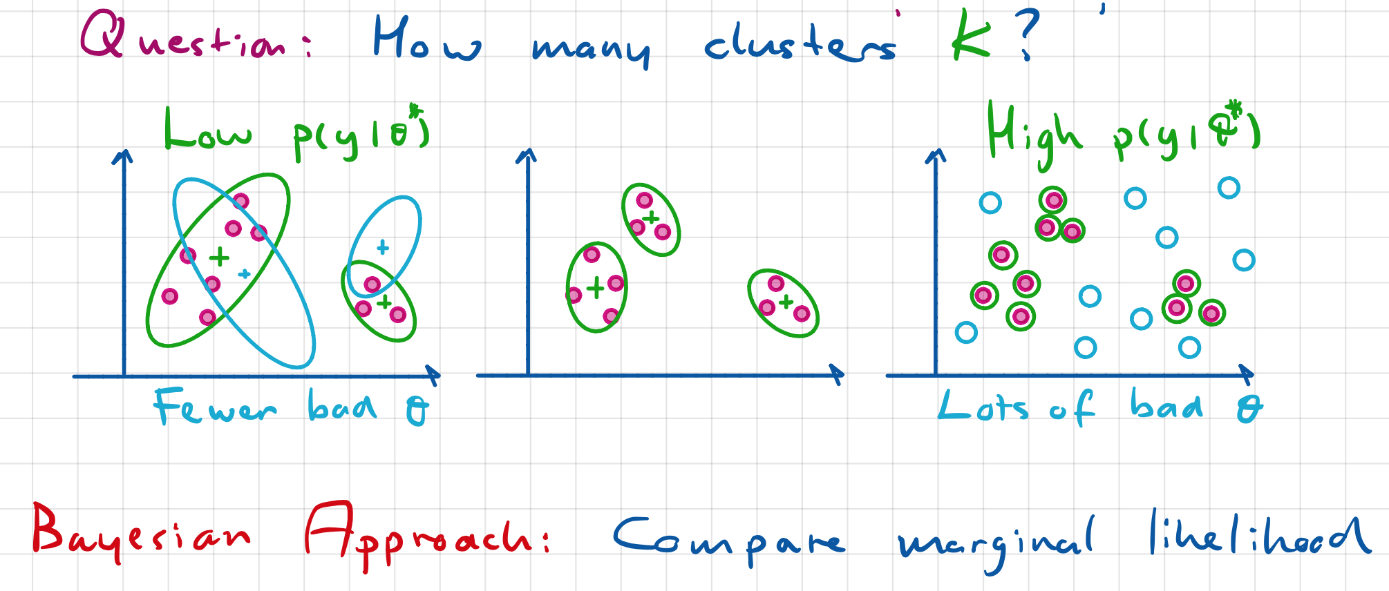
Suppose that we are doing clustering on the data points shown in the figure above, and we ask the question, “How many clusters K should I use?” In the first example, we try to fit 2 clusters to the data, in the second example, we try 3 clusters, and lastly, we try 10 clusters. If we look at the likelihood of the data given the parameters, then the last example has a really high likelihood, p(y|\theta), but the first example has low likelihood. Even though the last example has high likelihood, we also know that the clusters are over-fitting. The question is, can we describe in math what over-fitting looks like?

The intuition is: If we randomly drew new clusters for the data, how likely is it that the clusters would be on top of the data? For the last example, the probability is next to zero. On the other hand, for the first example, some of the points would probably fall into the new clusters (shown in blue). We can formalize that by looking at the marginal likelihood, which is p(y|k) (probability of y given the number of clusters k).

K^* = \underset{{k \in {1, ... , K^{max}}}}{\text{argmax}} p(y|k) = \underset{k}{\text{argmax}} \int d\theta p(y|\theta)p(\theta |k)

where p(\theta |k), describes the probability of the positions of the clusters given the number of clusters. We are going to go from K=1 cluster to the max number of clusters, and for each of those, we are going to compute the integral. We can think of the marginal likelihood as the Best Average Fit for the data!
Comparing Importance Sampling with MCMC

So now we know why having the marginal likelihood is kind of a big deal. However, Importance Sampling has an annoying property that makes it hard to generate a bunch of good samples. Consider the example we just discussed. Importance Sampling would basically randomly guess where to put clusters, which wouldn’t be efficient. MCMC, on the other hand, has this nice property where if we have a bad sample, we have a transition kernel that can give us a new sample. If the new sample is better, then we keep it. So if we keep getting better and better samples, we are more likely to get more good samples than when we randomly guess (like in Importance Sampling).

So the question now is “Why not both MCMC and IS?“

Annealing Importance Sampling

Idea 1 (Importance Sampling)

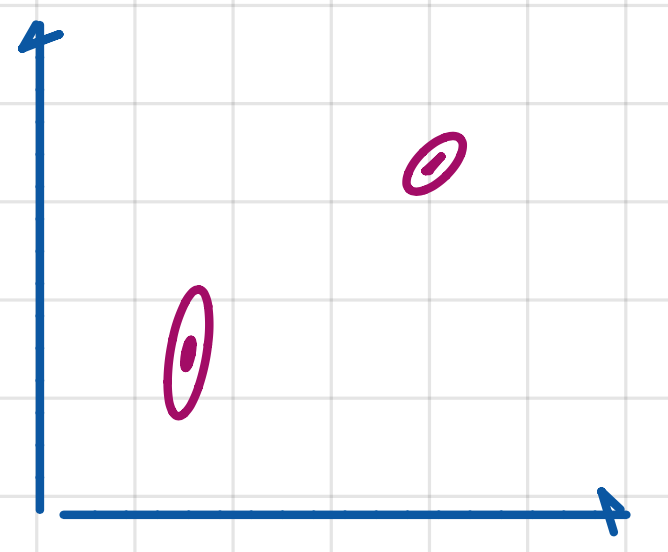
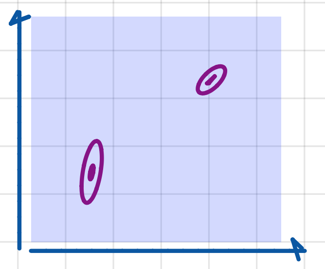
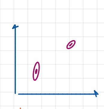
Imagine that we have we have two tiny clusters (above on the left), and we decide to sample uniformly from the shaded square within the plot (right). It would actually take a very long time to get sufficient samples that lie within the two tiny clusters. So the question we ask here is, “Can we make this problem a little bit easier?” How can we make it easier?

Well, imagine that we take the small cluster and make it a little broader. Then, we take those broader clusters and make those broader, and we keep going until we get a large single cluster.

We end up with something that can easily sample from! But how can we make this happen… and how does really solve our initial problem? Well, what if we could get samples from the broadest cluster and then refine those samples to get samples from a less broad cluster… and keep going until our samples are so refined and come from the original two small clusters?

That seems like a good idea, right!?

Idea 1: Break the problem into simple problems. Specifically, sample via intermediates of distributions.

Let’s say that our end goal is get some joint probability, p(y, \theta) of some data, y, and latent variables, \theta (which can be model parameters). However, we also want a really easy distribution to start with. Well, the easiest probability distribution we can is use is the prior, p(\theta). It’s easy because sampling from the prior doesn’t require any inference.
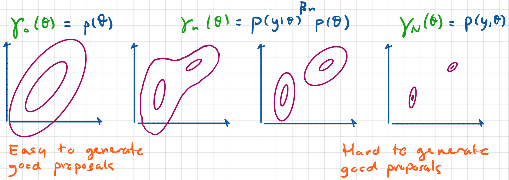

So now the question is, “what can we do so that we start at the easy distribution and smoothly transition to the final (and hard) joint distribution?”

Let’s think about this! The relationship between the prior and the joint probability is that the joint probability is equal to the likelihood times the prior:

p(y, \theta) = p(\theta \mid y) p(\theta)

So what really let’s us start from the prior and end up to the joint probability is the likelihood! We basically remove the likelihood from the joint probability and then gradually add it back in.

One way we can do this is by introducing a number, \beta_n, where we use it to get the n^{th} intermediate distribution:

p(y  \mid \theta)^{\beta_n} p(\theta)

If \beta_n = 0, what do have? We are left with just the prior. If \beta_n =1, we have the full joint distribution. So to get a sequence of intermediate distributions, we pick a sequence of values that smoothly go from 0 to 1.

Idea 2 (Transition Kernels)

Now that we know how to get intermediate distributions, let’s talk about how we can use them.

Before we move on, let’s think about the overall goal again. We started off with an example showing that we want to learn clusters for some data, y. If we are using Gaussian distributions to represent our clusters, then our parameters, \theta, would be the mean and standard deviation, \theta = {\mu, \sigma^2 }. Therefore we are trying to learn the cluster means and standard deviations to best represent the data.

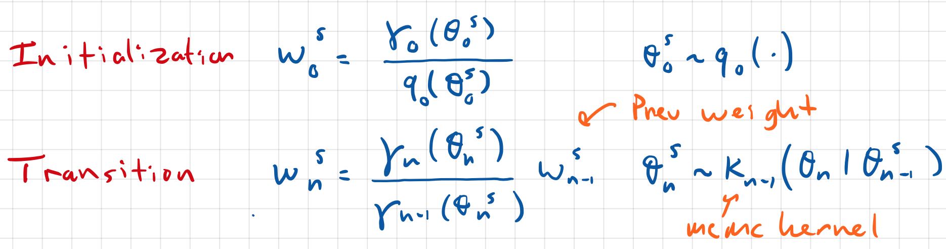
Initialization

Let’s begin by saying that we will sample a first sample from some proposal distribution: \theta_0^s \sim q(\cdot) (using a zero to signify the first sample we have). The sample is going to have an importance weight: w_0^s = \frac{\gamma(x_0^s)} {q(x_0^s)}, (just like in Importance Sampling).

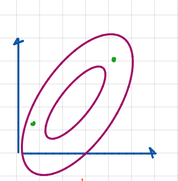
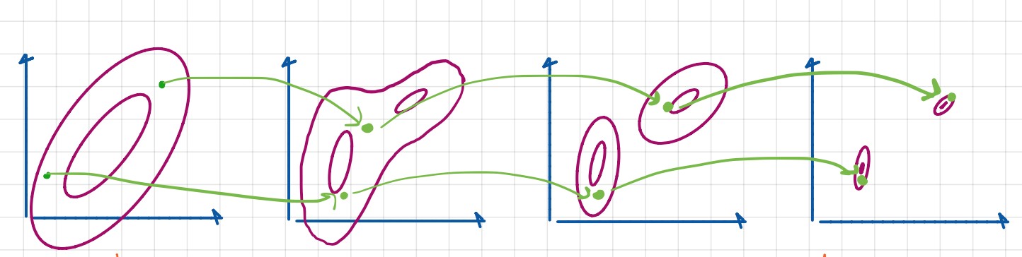
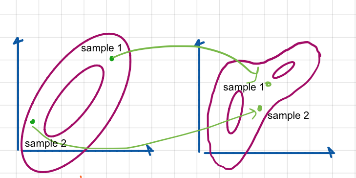
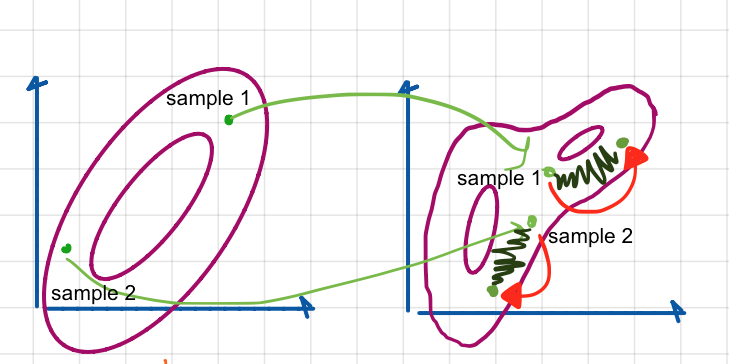
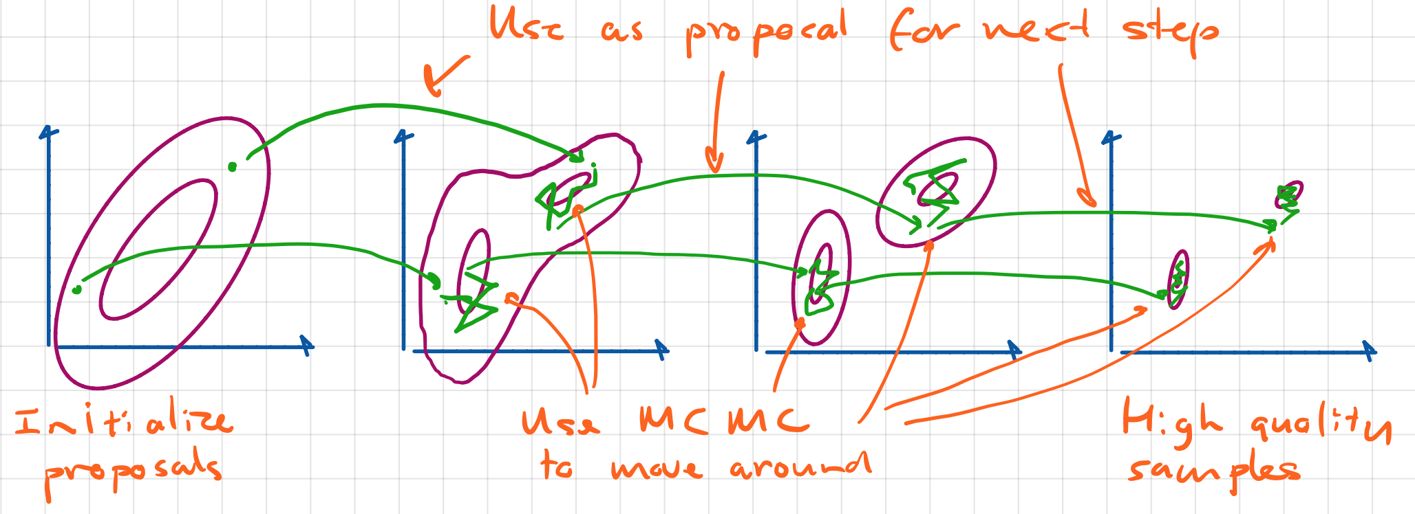
Now image that we have two samples (as shown in the figure above in green and within the prior distribution, \gamma_0(\cdot). So now what we want to do is evaluate those samples relative to the next (and new) density, \gamma_{n+1}(\cdot).

To do that, we are doing to use some form of transition kernel (just like in MCMC) to move the samples within the new density. We can move it several times. This gives us a new sample within the new density.

\theta_n^s \sim k_{n-1}(\theta_n \mid \theta_{n-1})

However, this means that we have a new importance weight for these new samples. The new weight, w_n^s, is updated as follows (I will derive it in a moment):

w_n^s = \frac{\gamma_n(\theta_n^s)}{\gamma_{n-1}(\theta_n^s)} w_{n-1}^s

So you can imagine now doing that for all of the intermediate distributions until we get to the final one. The algorithm is rather straightforward from here: 1) sample from some initial proposal, 2) get an importance weight, 3) evaluate the sample at the next density which gives you a new importance weight, 4) move the sample around the new density, then 5) repeat to the following density.

Understanding Idea 1: Deriving New Importance Weights

So how do we end up with the equation of the new weight evaluated at the next density? To answer this, let’s begin with a valid importance weight. Let’s assume that we sampled from a normalized density, x \sim \pi(x)_{n-1}, and we have an unnormalized density at the next step, \gamma_{n}(x). Then a reasonable importance weight would be:

w_n = \frac{\gamma_n(x)}{\pi_{n-1}(x)} \qquad x \sim \pi_{n-1}(x)

We know that the relationship between a normalized density and an unnormalized density is the normalization constant, Z, where \pi_n = \frac{\gamma_n(x)}{Z_n}. Then one way we can rewrite w_n is:

w_n = \frac{\gamma_n(x)}{\pi_{n-1}(x)} = \frac{\gamma_n(x)}{\gamma_{n-1}(x)} Z_{n-1} \qquad x \sim \pi_{n-1}(x)

Now imagine instead of sampling from \pi_{n-1}(x), we sample from \pi_{n-2}(x). Then we’d have:

w_n = \frac{\gamma_n(x)}{\pi_{n-2}(x)} \qquad x \sim \pi_{n-2}(x)

Then if we use the multiplying by 1 trick on this, 1 = \frac{\gamma_{n-1}(x)}{\gamma_{n-1}(x)}. We have

w_n = \frac{\gamma_n(x)}{\pi_{n-2}(x)} =   \frac{\gamma_n(x)}{\gamma_{n-1}(x)} \frac{\gamma_{n-1}(x)}{\pi_{n-2}(x)} \qquad x \sim \pi_{n-2}(x)

Notice how \frac{\gamma_{n-1}(x)}{\pi_{n-2}(x)} = w_{n-1} ! Therefore we can write:

w_n = \frac{\gamma_n(x)}{\gamma_{n-1}(x)} w_{n-1}  \qquad x \sim \pi_{n-2}(x)

This is really nice for us because now all we have to do to get a new weight is relate it to the previous weight.

Understanding Idea 2: Transition Kernels

So now we talk about combining Importance Sampling with MCMC.

We start with an importance sampler which means we sample from a proposal and then we get an importance weight. Now, MCMC let us move the sample around using a transition kernel, \kappa(x' \mid x) (assuming it satisfies detailed balance).

w = \frac{\gamma(x)}{q(x)} \qquad x \sim q(x) \qquad x' \sim \kappa(x' \mid x)

We know that we update the importance weight relative to a new density, but do we need to update our weight after moving our sample around in the new density? Well, let’s think a little bit.

w' = \:?

Let’s remember what an importance weight looks like: w = \frac{\gamma(x)}{q(x)}. So getting some \gamma and q for our w' would mean considering both x and x'. Let’s expand on that starting with the proposal.

The proposal mechanism here is really doing two things at once, getting x and x', \tilde{q}(x, x'). This is done as shown before, sampling from some proposal and then using a transition kernel.

\tilde{q}(x,x') = q(x)\kappa(x'\mid x)

The unnormalized density also considers both x and x', \tilde{\gamma}(x, x').

\tilde{\gamma}(x,x') = \gamma(x')\kappa(x\mid x')

So then our new weight would look like:

w' = \frac{\tilde{\gamma}(x,x')}{\tilde{q}(x,x')} = \frac{\gamma(x')\kappa(x\mid x')}{q(x)\kappa(x'\mid x)}

If our kernel satisfies detailed balance, \gamma(x)\kappa(x'\mid x) = \gamma(x')\kappa(x\mid x') … notice how if we rewrite our detailed balance equation to solve for \gamma(x), we will have \frac{\gamma(x')\kappa(x\mid x')}{\kappa(x'\mid x)} = \gamma(x). Our new weight now looks like:

w' = \frac{\gamma(x')\kappa(x\mid x')}{q(x)\kappa(x'\mid x)} = \frac{\gamma(x)}{q(x)} = w

which equals to the original importance weight we calculated when we evaluated the sample on the new density!

So back to the original question here: do we need to update our weight after moving our sample around in the new density? The answer is nope! This is neat because we use MCMC on each distribution while preserving the importance weights!

MCMC: Metropolis-Hastings

This blog is a continuation of the previous discussion on MCMC, What are Monte Carlo Markov Chains (MCMC)? I introduce a well known MCMC algorithm, Metropolis-Hastings (MH).  I describe how MH behaves and prove how it holds detailed balance. Then I show an example of a bad proposal, and move on to show what generally people choose for good proposals. I close with a brief comparison of MCMC and (Self-Normalized) Importance Sampling.

Before we start, I’d like to thank Jan-Willem van de Meent for his lectures in his Advance Machine Learning Class for PhD students at Northeastern University. The images shown are from his lectures. In addition, I’d like to address that more details on MC algorithms can be found in An Introduction to Probabilistic Programming available [arXiv]. This book is intended as a graduate-level introduction to probabilistic programming languages and methods for inference in probabilistic programs.

It turns out that it’s not so easy to design a transition operator that guarantees to have detailed balance. But what if maybe we can use something that turns any proposal operator (which is something we can come up with) into something that satisfies detailed balance. This folks, is what Metropolis-Hastings does for us!

What is Metropolis-Hastings?

The intuition behind Metropolis-Hastings is that

  1. We know we need to have an operator that satisfies detailed balance
  2. We can propose something ( some sample x')
  3. We can check whether the proposal is good or not
  4. And sometimes we are going to keep that proposal, and sometimes we are not…. in such a way that keeping it vs not keeping it satisfies detailed balance.

Now I’ll introduce mathematically how MH works and then discuss why it works.

We begin with a current sample, x^s, which we will use to get a new sample, x^{'} using a proposal distribution, q(x' \mid x^s). The notation looks as follows: x' \sim q(x' \mid x^s).

Then we decide to keep the new sample, x^{s+1} = x' with probability:

\alpha = \min\left(1, \frac{\pi(x')q(x^s|x')}{\pi(x^s)q(x'|x^s)}\right)

To discuss what this probability actually means, let’s remind ourselves what the detailed balance relationship is. It is: \pi(x)p(x'|x) = \pi(x')p(x|x'). But since we are now working with proposals, let’s switch notation from p to q.

\pi(x)q(x'|x) = \pi(x')q(x|x')

Side Note: Sometimes transition probabilities such as q(x \mid x') can be referred to as a kernel. Instead of being specific with what is making the transition, we generalize by saying we are using a transition kernel. Common notation is \kappa(x \mid x'). They both represent getting one sample dependent on another sample.

Let’s suppose that q(\cdot) satisfies detailed balance, then the ratio here between \pi(x)q(x'|x) and \pi(x')q(x|x') is 1. So now let’s refer back to the probability:

\alpha = \min\left(1, \frac{\pi(x')q(x^s|x')}{\pi(x^s)q(x'|x^s)}\right)

Here we are saying that with probability \alpha, we are going to set the proposal to our new sample, x^{s+1} = x', and with probability (1 - \alpha) we are going to reject the proposal. When we reject the proposal, our next sample is set to the same sample as before, , x^{s+1} = x.

We see that if \alpha = 1, we always accept the proposal. Basically, if our transition kernel always satisfies detailed balance, we can always accept it!

However, if it does not satisfy detailed balance, then this means that somehow there’s an imbalance with the kinds of proposals we are getting. There are some kind of samples that we are proposing too often and other kinds that we are not proposing often enough.

Question: if the ratio \frac{\pi(x')q(x^s|x')}{\pi(x^s)q(x'|x^s)} is larger than 1, does this mean we are proposing some kind of samples too often or not often enough?

Let’s think about it! If we are not proposing the kind of samples we want more, then we should probably accept them with higher probability. However, if we are seeing a sample too often, then maybe we should only accept it sometimes. Therefore if \frac{\pi(x')q(x|x')}{\pi(x) q(x'|x)} > 1, it’s because we are seeing a rare sample we want more of (we are proposing not often enough). However, basic probability tells us that probabilities max out at 1. This is why we add the \text{min} to get the probability \alpha.

So what does Metropolis-Hastings do for us? It’s an algorithm that basically corrects our proposals in order to preserve detailed-balance! Neat, huh?

Proving Detailed Balance for Metropolis-Hastings

The idea behind Metropolis-Hasting is that we can get a new (transitioned/dependent) sample when we sample from a proposal, x' \sim q(x'|x^s), and get our next sample, x^{s+1} = x' with probability \alpha = \min\left(1, \frac{\pi(x')q(x|x')}{\pi(x)q(x'|x)}\right), otherwise we keep our previous sample, x^{s+1} = x^s.

When we have this particular sampling scheme, we an have an implied transition kernel that can tell us (when we have x and x'), what is the probability that we are going to see a transition from x to x'. In order to reason about this, we need to consider two cases. It could be that x' is not the same value as x, but they could be in fact the same value where x = x'. We formulate this by working backwards.
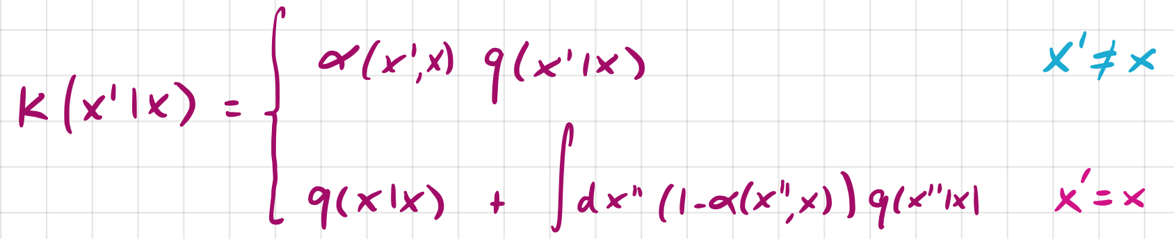
In the figure above, we show that in order to get a value x \neq x', we first need to sample an x' from q(x'|x) and then we need to decide to keep the sample with probability \alpha. Therefore for the case where x \neq x', we have \alpha * q(x'|x).

Note that there are two cases where x = x' and \alpha = 1. The first is if somehow we were able to sample the exact same sample x again (this can only happen in some cases, for example if we are sampling from a Bernoulli distribution, but if we were sampling from a Normal, then it would be very unlikely). This gives us \alpha * q(x|x) = q(x|x). The second possibility of getting the same sample again is by rejecting. Then we calculate the probability that any rejected sample will give us the same sample as before. We integrate over possible values we could have rejected, x'', and then we write the probability of (1 - \alpha'')q(x''|x).

We can prove detailed balance once we write out the kernel like this quite easily because it splits the problem into two small proofs, one for the case where x = x' and another for x \neq x'.

In the case where x = x, we can just say: \pi(x)\kappa(x|x) = \pi(x)\kappa(x|x)

Really in MH, the point is not to describe how often we stay at the sample (there are other properties that should help this from happening), but rather how often we transition from sample to sample. Therefore we care more about the next case.

In the case where x = x', we can say:

\pi(x)\kappa(x'|x) = \alpha q(x'|x)\pi(x) \qquad \text{replace } \alpha \text{ with } \text{min}\left(1, \frac{\pi(x')q(x|x')}{\pi(x)q(x'|x)}\right)

= \text{min}( \pi(x) q(x'|x), \pi(x')q(x|x'))

= \text{min}( \pi(x') q(x|x'), \pi(x)q(x'|x))

= \alpha q(x|x')\pi(x')

= \pi(x')\kappa(x|x')

\pi(x)\kappa(x'|x) = \pi(x')\kappa(x|x')

Unnormalized Densities

Now we know that Metropolis-Hastings preserves detailed-balance. It is also the case that once you have detailed-balance, you can say if you have a normalized density, \pi, then

\pi(x) = \frac{\gamma(x)}{Z} \text{ and } \pi(x') = \frac{\gamma(x')}{Z}
\frac{\pi(x')}{\pi(x)} = \frac{\gamma(x')}{\gamma(x)}

In practice, when doing MH, this is a nice property because we don’t always have the normalized density. we can calculate the acceptance probability using the unnormalized density, \gamma(x).

\alpha = \min(1, \frac{\pi(x')q(x|x')}{\pi(x)q(x'|x)})
= \text{min}(1, \frac{\gamma(x')q(x|x')}{\gamma(x) q(x'|x)})
\text{For a Bayesian Inference Example where } \gamma(x)  = p(y,x)
= \text{min}(1, \frac{p(y,x')q(x|x')}{p(y,x) q(x'|x)})

It’s important to note that MH is very general. We can design any transition proposal and if that proposal violates detailed-balance then we can use the Metropolis-Hastings’ acceptance ratio to clean up the mis-designed proposal. We have shown that we can always evaluate the ratio whenever we have an unnormalized density and don’t have the normalize density (which is always the case).

Example of a Bad Proposal

We can do likelihood weighting. Suppose that we have to sample x' | x. We can sample from the prior, which means that we can ignore was x was.

q(x'|x) = p(x') \;\;\;\;\; \text{(Independent from previous sample)}

This is what we call Independent Metropolis-Hastings because new samples are independent from the previous sample (which is valid). Now we can see what our new acceptance ratio is:

\alpha = \text{min}(1, \frac{p(y,x')q(x|x')}{p(y,x) q(x'|x)})
= \text{min}(1, \frac{p(y,x')p(x')p(x)}{p(y,x)p(x)p(x')})
= \text{min}(1, \frac{p(y,x')}{p(y,x)})

Because our probabilities cancel, we are left with the ratio of the likelihoods. But we have the same issue as the likelihood weighting where we have low acceptance probabilities. With the exception that this sampler won’t let go of a good x, this is no better than doing likelihood weighting because we still have to wait until we get a good sample again.

More Common Examples of Choosing Proposals

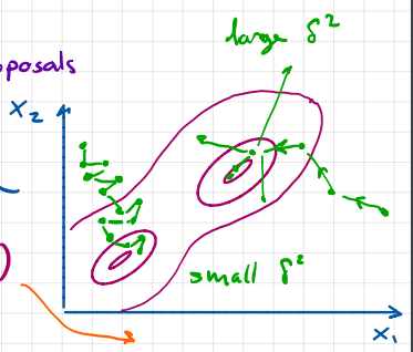
It’s much more common to setup a proposal where we sample a new sample, x', from a Normal distribution centered on x with some standard deviation, \delta^2. It’s important to note that \delta^2 is symmetric. This means that the probability going from x' to x should be the same as the probability as going from x to x', or q(x'|x) = q(x|x').

This makes our acceptance ratio a bit easier since q(x'|x) = q(x|x')

\alpha = \text{min}(1, \frac{\gamma(x')q(x|x')}{\gamma(x) q(x'|x)})
= \text{min}(1, \frac{\gamma(x')}{\gamma(x)})

What are the options for our step size, \delta^2? (1) We can take really small steps. This means we will then need a lot of steps to get somewhere (2) We can also take really large steps. However, we will probably jump around too much end up with samples we will more often reject.

So the question is then, How should we set our step size?

Based on people who have done some analysis, we should tune our acceptance rate. We keep adjusting it until we get a magic number, which is \alpha \approx 0.234. This is optimal under a set of assumptions. In practice, we want anything between 0.1 and 0.7 depending on what we are doing.

Summary – MCMC vs. Importance Sampling

We have looked at two MC samplers, MCMC and Importance Sampling.

For Importance Sampling we say: if we design some proposal, generate some samples, assign each sample a weight, we can now take the weighted-average over the samples. In particular, we know that the samples gives us an estimate of the marginal likelihood.

w^s = \frac{\gamma(x^s)}{q(x^s)}, \qquad x^s \sim q(x) \qquad E[w^s] = p(y)

For Metropolis-Hasting we do something different: We say, suppose we have a sample x^{s-1}. Now we are going to propose a new sample, and are going to pick a number between 0 and 1. We are going to calculate the acceptance ratio, and if my number is larger than my acceptance ratio then I keep the previous sample otherwise I keep the new sample.

MCMC has a transition probability/kernel x^s \sim \kappa(x\mid x^{s-1}) and satisfies detailed balance \pi(x^s)\kappa(x^{s-1}\mid x^s) = \pi(x^{s-1})\kappa(x^{s}\mid x^{s-1}).

The difference: is that IS gives us the estimate of our marginal, and MH allows us to do hill-climbing, but doesn’t give us an estimate for the marginal.

We’ll discuss why having an estimate for the marginal is important when we discuss Annealed Importance Sampling!

Thanks for reading!

What are Monte Carlo Markov Chains (MCMC)?

In this blog, I introduce what a Monte Carlo Markov Chain (MCMC) is and discuss how MCMC is different from Importance Sampling. I discuss what a homogeneous Markov Chain is and what convergence means for MCMC. Lastly I discuss detailed balance and how good transition probabilities for Markov Chains satisfy this property.

Before we start, I’d like to thank Jan-Willem van de Meent for his lectures in his Advance Machine Learning Class for PhD students at Northeastern University. The images shown are inspired by or exactly from his lectures. In addition, I’d like to address that more details on MCMC algorithms can be found in An Introduction to Probabilistic Programming available [arXiv]. This book is intended as a graduate-level introduction to probabilistic programming languages and methods for inference in probabilistic programs.

Why Move On from Importance Sampling?

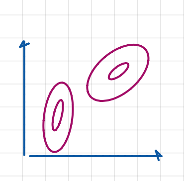
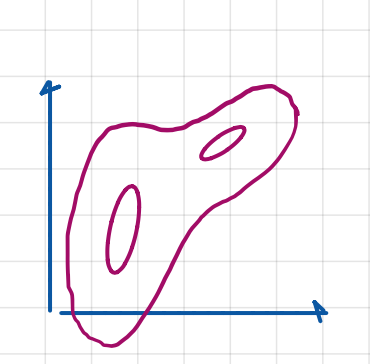
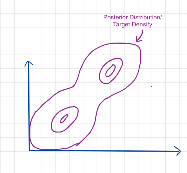
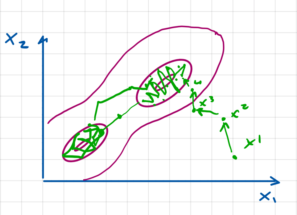
Imagine that we have a distribution like in the example drawn on the left (in purple). The distribution is bimodal, meaning that there are two areas of concentration.

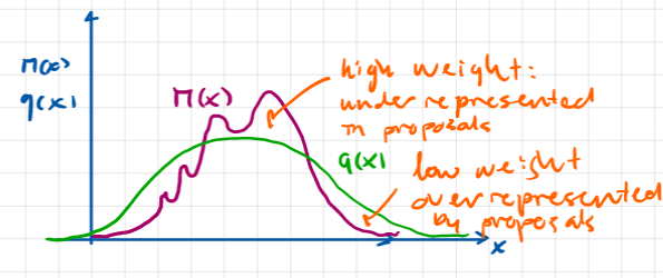
If we were to use Self-Normalizing Importance Sampling (SNIS) to get samples from this distribution (see my last blog on Importance Sampling vs Self-Normalizing IS), we would draw samples from the proposal distribution and either keep it if the importance weight is high, or throw it away if the weight is low.

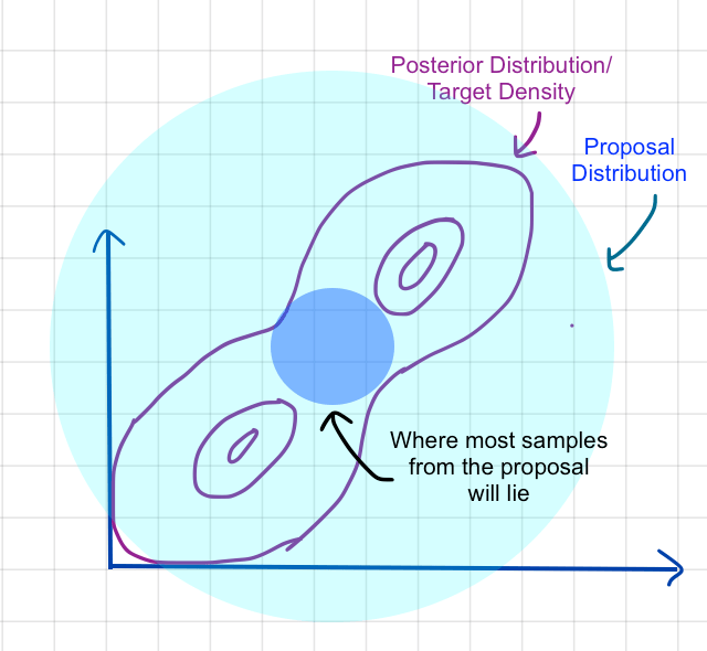
Imagine we have a Gaussian proposal distribution that covered the entire purple density. If the mean of the proposal distribution overlaid in between the two modes in the purple density, most samples drawn would have a low importance weight (keep in mind that samples from a Gaussian distribution center around its mean). In this case, we would probably throw away a lot of samples since we specifically want more samples that are within the two concentrated areas of the distribution.

Why is throwing away so many samples bad? Ideally, we want to get as many good samples as possible because the more we have, the better we can know what the posterior distribution looks like. However, realistically, we work with high-dimensional problems. The number of samples we need exponentially increases as the number of dimensions increase. Imagine getting 1000 samples and throwing away 990. 10 good samples is definitely not enough to describe a posterior distribution of high dimensionality.

The question is, how do we move away from the idea of throwing away a lot of samples? Instead, is there a way that we continue to get similar good samples once we have a good sample already? We can, using MCMC.

Monte Carlo Markov Chain (MCMC)

Monte Carlo Markov Chains move on from the idea of randomly sampling from the proposal. Instead MCMC introduces the idea of getting similar samples to already good samples, i.e. start with a sample we previously drew, x^{s-1}, now use it to propose a new sample nearby x^{s}.

Markov Chains

Having a chain means having a sequence, X^1, ... , X^S where S is the total number of samples. The Markov property says that instead of getting a new sample based on all of the previous samples, we can get a new sample just based off the previous (single) sample.

X^s | X^{s-1} ... \perp\!\!\!\perp X^1, ... X^{s-2}

where \perp\!\!\!\perp means conditionally independent

p(x^s|x^{1:1-s}) = p(x^s|x^{s-1})

What is an example of something that is not a Markov Chain? Consider words in a sentence. Each word in a sentence is not a Markov Chain since each word does not depend on only the previously said word, but instead on several previous words, or even previous sentences.

Homogenous Markov Chains

Additionally we are going to talk about a specific kind of Markov Chain, a homogeneous Markov Chain. The best way to describe what a homogeneous chain is to start with what is not a homogeneous chain. Let’s consider a sentence with words again. Let’s say you’re generating a sentence, most of the time, this process is non-homogeneous. This is because the conditional distribution changes as you keep generating words.

In order for a chain to be homogeneous, we have to use the same conditional distribution for the next step of the sequence. We see this idea in hidden Markov models. At each time we are at a state, we decide whether to go to another state or not. If we decide to not to go another state, at the next step, we decide again. When we keep doing that, we get a sequence where we keep flipping back and forth between states. So the prior probability there at each time of flipping states, is exactly the same. That is an example of a homogeneous Markov chain.

A Markov chain is homogeneous when we have the same transition distribution for every sample s:

p(X^s= x^s|X^{s-1}=x^{s-1}) = p(X^2=x^s|X^1=x^{s-1})

This simply means we use the sample probability to move around!

Convergence

Now that we have talked about a homogeneous Markov chain, I’ll discuss convergence towards the target density (another term for posterior or true distribution). Ideally, we want to converge to this target density, which we will refer to as \pi(x). We can basically start looking at a limit of more and more samples and the probability that sample s takes on a particular value x. If we continue taking samples long enough, we want that probability to be exactly the same as the probability that some random variable under the target density takes on.

\lim_{s\rightarrow \infty} p(X^s=x) = \pi(X=x)

What’s the intuition behind convergence here?

Let’s refer to the figure above. Let again consider the purple distribution. This will be the target density we wish to converge to. Remember that there are two modes to this density; there are two regions of high probability. Let’s initialize a Markov chain with x^1 being our first sample. If we keep transitioning to new points, x^2, ... x^S, you can image that we are doing some form of random walk. If we run our random walk long enough, then we hope that all these points in this random walk will visit each region within the space proportional to the target density. So regions of high probability are places we want our random walk to visit more often than those of low probability.

Detailed Balance

Now, notice how I haven’t really said anything yet, other than if we have a Markov chain, we are picking where to go next given a previous step. Also, I have said that if we design a good Markov chain, then maybe we can converge towards the target density.

I will now introduce what sort of Markov chains might converge to this target density. I’ll introduce a transition operator where if we already have a sample from the target density then that means we are going to stay at the target density. Remember that this is the idea behind MCMC that makes it different from Importance Sampling.

NOTE: We are going to do some hand waving and say that if we leave the target density invariant, it also converges. I won’t prove that here because it’s a bit of a pain. We will simply gloss over that theoretical aspect here, but I will introduce the notion of leaving a target density invariant.

The Markov Chain we will talk about is one that satisfies detailed balance. A homogeneous Markov Chain satisfies detailed balance when

\pi(x)p(x'|x) = \pi(x')p(x|x')

This says, suppose we have the density at x, \pi(x), and we define a probability of going to the variable x' given that I was at x. We say that this quantity should be same as the quantity of starting at x', \pi(x') and defining the probability of going to x from x'.

Another way to say this is for every pair x and x', our sampling mechanism p(x'|x) leaves \pi(x) invariant:

Since \int dx' p(x'|x) = 1, (multiply by 1 trick!) we can write

\pi(x)\ = \int dx' \pi(x) p(x'|x)

Then by definition (\pi(x)p(x'|x) = \pi(x')p(x|x')) we can rewrite \pi(x) as

\pi(x) = \int dx' \pi(x') p(x|x')

So what does this really mean? It means that if I start with a distribution of \pi(x) and look at all possible ways we can end up at a given point x, starting from some other point, x', and we take the expectation of how often we start at some x', then we also get \pi(x).

So if we start with x', x' \sim \pi(x), and use it to get a new sample from the transition probability, x \mid x' \sim p(x\mid x'), then I have just sampled x from \pi(x), x \sim \pi(x).

Side Note: Even though using the transition probability means x\sim \pi(x) and x' \sim \pi(x), using the transition probability means that x and x' are not independent samples.

Now we can say that good Markov Chains have transition probabilities that satisfy this property, detailed balance!

Thanks for reading!

Importance Sampling (IS) vs Self-Normalized IS

I begin by discussing why Monte Carlo Estimators are used. One Monte Carlo Estimator I introduce is Importance Sampling. Most of the time, however, Importance Sampling alone is not enough. Instead we resort to using Self-Normalized Importance Sampling. In this blog, I discuss what we really mean when we say Importance Sampling. We learn that, generally, when someone says they are using Importance Sampling, they are really mean Self-Normalized Importance Sampling.

Before we start, I’d like to thank Jan-Willem van de Meent for his lectures in his Advance Machine Learning Class for PhD students at Northeastern University. The images shown are from his lectures. In addition, I’d like to address that more details on MC algorithms can be found in An Introduction to Probabilistic Programming available [arXiv]. This book is intended as a graduate-level introduction to probabilistic programming languages and methods for inference in probabilistic programs.

Monte Carlo Estimators

I’d like to begin by stating that Importance Sampling is a Monte Carlo Estimator. Our goal for a Monte Carlo Estimator is to calculate the expectation of some function with respect to the normalized density \pi(x) where

\pi(x) = \gamma(x) / Z \\ = P(y, x) / P(y) \\ = P(x | y) \\

\gamma(x) is an unnormalized density which we can sample from and Z is a normalizing constant

Z = \int dx \gamma(x) \\ = \int dx P(y, x) \\ = P(y)

F = E_{\pi(x)}[f(x)] \\ = \int dx \pi(x) f(x) \\ = E_{p(x|y)}[f(x)]

Why do we use Monte Carlo Estimators?

We use Monte Carlo Estimators because we do not have access to the normalized density, \pi(x). Having access to the normalized density requires us to compute the normalizing constant, Z, which means integrating over all possible values \gamma(x) could evaluate to. This is what we (almost always) cannot do! The good news is that we do have access to the unnormalized density, \gamma(x).

The key idea here is that we use samples from the unnormalized density, \gamma(x) to estimate some function we are interested in learning. We assume here that samples from \gamma(x) are independent and identically distributed, (IID).

\hat{F}^S = \frac{1}{S} \sum_{s=1}^{S}f(x^s) \ x^s  \sim \pi(x)

There are two main properties that Monte Carlo Estimators hold. The first is that the estimate is unbiased. The second is that it is consistent. I’ll briefly describe what each mean.

The estimate is unbiased when the expected value of the estimator is the exact quantity we are trying to estimate.

E[\hat{F}^S] = E[ \frac{1}{S} \sum_{s=1}^{S} f(x^S)] \\ = \frac{1}{S} \sum_{s=1}^{S} E[f(x^S)] \\ = E [f(x^S)] \\ = F

Our estimator is consistent when the estimation becomes more accurate as we use more samples. This happens when the variance approaches zero as the number of samples approaches infinity:

\lim\limits_{S \rightarrow \infty} E \left[(\hat{F}^S - F)^2\right] = 0.

Importance Sampling

When we use importance sampling, we try to find the best estimate we can by guessing! We ask, what is a distribution that can give me samples that might also be samples from the distribution we actually care about, \pi(x)?

The distribution we use to make guesses is what we call a proposal distribution, q(x). If we look at the figure below, we see an example of what a normalized distribution (also called the true or posterior distribution) might look like drawn in purple, and what a guessing distribution looks like drawn in green (a gaussian in this case).
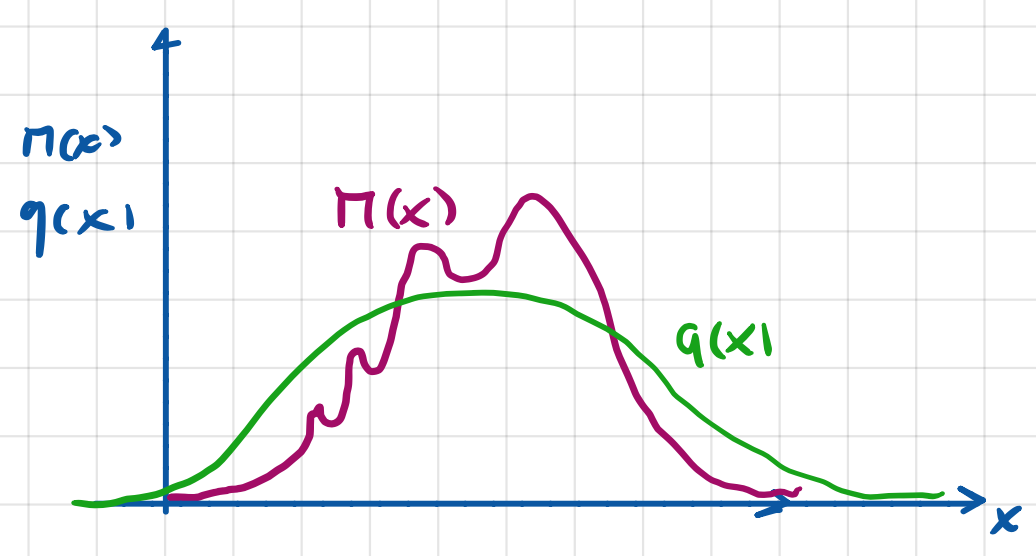
We expect \pi(x) to be a distribution that is difficult to describe, that is why it has so many wiggles in this example. As for the guessing distribution, the proposal distribution, q(x), it is generally a very simple distribution we know how to sample from. That is why we commonly use Gaussian distributions as proposal distributions.

The idea behind importance sampling is that we can measure how well a sample from the proposal does with respect to the posterior distribution. We can measure using an importance weight, w.

To get an intuition of what high and low importance weights mean, let’s refer to the example again. Let’s say we get a sample, x, and it is evaluated by both the proposal, q(x), and posterior, \pi(x), distributions ( I will now stop using the word distribution when referring to the proposal and posterior distributions).

Consider two cases.

  1. The sample lands outside the proposal, but inside the posterior.
  2. The sample lands inside the proposal, but outside the posterior.

In the first case, we get samples that are under represented by the proposal, thus producing higher importance weights!

In the second case, we get samples that are overrepresented by the proposal, which yields low importance weights!

The goal here is get samples that better represent the posterior. The higher the importance weight, the better it approximates a sample from the posterior.

More High-Weighted Samples = Better Approximation of Posterior Distribution

NOTE: q(x) must have the same or a larger support than \pi(x).

Let’s now show this using math.

Remember that with a Monte Carlo Estimator, we want to approximate some function. E_{\pi(x)}[f(x)] = \int dx \pi(x) f(x)

We can play around with this equation in order to make it more useful. We do this by using a trick we often use in machine learning, multiplying by 1! Our 1 we multiply here is \frac{q(x)}{q(x)}. So now we have:

\int dx \pi(x) f(x)  = \int dx q(x) \frac{\pi(x)}{q(x)} f(x)

As part of being an estimator, we can approximate this integral using samples:

E_{q(x)}[f(x)] \approx \frac{1}{S} \sum_{s=1}^{S} \frac{\pi(x^S)}{q(x^S)}f(x^S), \; x^S \sim q(x)

\frac{\pi(x^S)}{q(x^S)} is what we call the importance weight, w.

And there you have it, Importance Sampling!

To do Importance Sampling, all you need is a proposal distribution you can sample from, x \sim q(x), in order to get an importance weight, w = \frac{\pi(x)}{q(x)}, that tells you how well it approximates being a sample from the posterior distribution, \pi(x).

We’re done! … or are we?

If you’re thinking, “Wait! but I thought we couldn’t evaluate a sample using \pi(x) because that requires us knowing the normalizing constant, Z! And if we can’t evaluate a sample at \pi(x), we can’t get an importance weight!”
…
and you would be right!

Folks, this is where I now introduce Self-Normalized Importance Sampling.

Self-Normalized Importance Sampling

As mentioned before, people usually refer to Self-Normalized Importance Sampling (SNIS) when they say Importance Sampling. Now, the question is, what makes SNIS better? The answer is, it’s more useful! Instead of relying on the normalized distribution, \pi(x) (which we do not know), we use something we do know: the unnormalized distribution, \gamma(x). But how? By using another Monte Carlo Estimator to estimate our normalizing constant, Z!

Remember that Z = \int dx \gamma(x) and \pi(x) = \gamma(x) / Z

If we rewrite \pi(x) = \gamma(x) / Z as \gamma(x) =  Z * \pi(x)

We can rewrite Z = \int dx\: \gamma(x) as Z =  Z \int dx\: \pi(x)

We can then do our multiply by 1 trick again, \frac{q(x)}{q(x)}!

Z = Z \int dx\: q(x) \frac{\pi(x)}{q(x)}
We can replace \pi(x)
Z = Z \int dx q(x) \frac{\gamma(x)}{q(x) Z}
Notice how the Zs cancel above on the right side!
Z = \int dx q(x) \frac{\gamma(x)}{q(x)}
This now looks like an expectation
we can turn into a Monte Carlo Estimator:
\hat{Z}^S = \frac{1}{S} \sum_{s=1}^{S} \frac{\gamma(x^S)}{q(x^S)} \:\: x^S \sim q(x)

Now to get Self-Normalized Importance Sampling, we combine the Importance Sampling estimator with the normalization constant estimator we just derived.

We update

E_{q(x)}[f(x)] \approx \frac{1}{S} \sum_{s=1}^{S} \frac{\pi(x^S)}{q(x^S)}f(x^S), \; x^S \sim q(x)

to

E_{q(x)}[f(x)] \approx \frac{1}{\hat{Z}^S} \frac{1}{S} \sum_{s=1}^{S}  \frac{\gamma(x^S)}{q(x^S)}f(x^S) \:\: x^S \sim q(x)

We can write this more neatly. Remember that we can define our weight as w^s = \frac{\gamma(x^S)}{q(x^S)}.

We can then rewrite our normalization constant estimate using this weight, \hat{Z}^S= \frac{1}{S} \sum_{s=1}^{S}w^S \approx p(y)

We can then write SNIS as

\hat{F}^S = \frac{1}{S \hat{Z}^S} \sum_{s=1}^{S} w^S f(x^S) = \sum_{s=1}^{S} \frac{w^S}{\sum_{s=1}^{S} W^S} f(x^S)

As you probably noticed, the weights are now normalized, hence Self-Normalized Importance Sampling!

Thank you for reading this blog!

Graphical Models in ML and How Easy it is to Break Conditional Independence

In this blog, I briefly introduce properties that graphical models have and the kinds we see in machine learning (ML). I introduce a simple problem with its graphical model and then work up to a more realistic example. I then demonstrate how easy it is for us to break conditional independence and discuss what that means for us.

Before we start, I’d like to thank Jan-Willem van de Meent for his lectures in his Advance Machine Learning Class for PhD students at Northeastern University. I use drawings from his lectures. In addition, I’d like to address that more details on graphical models can be found on David Barber’s book, Bayesian Reasoning and Machine Learning.

What Kinds of Graphs Do We Work With?

Let’s start off by briefly discussing three different properties graphs can have. This is important because graphs are used to define the problem we are going to work with. By introducing different kinds of graphs, we are exposed to the kinds of graphs most machine learning people work with. In most cases, designing a graph cleverly can make the difference between trying to solve a hard problem and a simple one.

Property 1: Directed vs. Undirected Graphs

These are graphs where the nodes are random variables. In the direct graph (left), we have directed edges whereas the undirected graph does not (right). It’s important to note that in either case, you can define the same density, p(a,b,c,d,e). It is common for us to care about how certain variables influence other variables (we’ll see a more concrete example of this in the examples below).
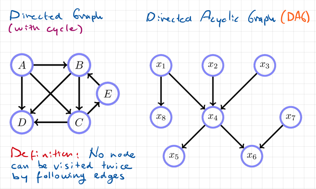
Property 2: Cyclic vs. Acyclic Graphs

How variables influence others is important. Our problem becomes more difficult if our graph contains cycles.

On the left, we can follow nodes A to B, B to C, C to E, and E back to B, this what called a cycle. On the right graph, we have an example of a graph that is acyclic. A graph that is acyclic and directed is known as a directed acyclic graph, or DAG. Most of the probabilistic models that we will discuss in machine learning will be DAGs. It should not be possible to visit a node twice by following the edges along the graph in a DAG.

Property 3: Connected Graphs

On the right, there are two paths to get to node f from node a, and on the left graph, there is only one path to get to f from node a. In most cases, we talk about graphs that are multiplely connected and are acyclic. It’s common to work with problems where a certain variable can affect another variable via different variables in-between.

Bayesian Network Examples

Now that we have discussed these basic properties, let’s make these ideas more tangible by discussing two examples of Bayesian Networks. The first will be a simple example taken from David Barber’s book mentioned above. The second will be a more realistic example using Naive Bayes.

Simple Example

Above we show an example of a Bayesian Network (sometimes called a Belief Network and Probabilistic Generative Model). Generally when referred as a Belief Network, it is a case where all of the random variables are binary. Each letter in the nodes (circles) have a meaning. Together they describe a situation, or a scenario. The graph above shows the nodes:

B Sherlock Holmes’ apartment was Burgled
A The Alarm went off
W Watson heard the alarm
G Mrs.Gibbon heard the alarm

where the edges show which variable influences other variables. For example, if the apartment was burgled, then that can cause the alarm to go off which can then be heard. This graph shows a way of breaking down the joint distribution into conditional distributions.

For example: Whether Mrs.Gibbon hears the alarm only depends on whether the alarm went off. It does not depend on whether Watson heard the alarm. So this is the distribution of B given A, p(B|A). The graph shows p(G, W, A, B) = p(G|A)p(W|A)p(A|B)p(B).

NOTE: What this graph does NOT say is what kind of random variables they are. It also does not say which type of distributions defines these conditional distributions. It only says these conditional distributions exist. So it’s not a full specification of a model, but it is a full specification of the structure of a model.

Given a graph like above, you can reason whether the apartment was burgled given that Watson and Mrs. Gibbson heard the alarm, this would give us a posterior

p(B|W, G) = \frac{p(G, W, B)}{p(W, G)} = \frac{\sum_{A} p(G,W,A,B)}{\sum_{A,B} p(G,W,A,B)}

where in order to find the posterior, we need to find p(G,W,B) which describes the marginal over A and p(W,G), the marginal over A, B.

Realistic Example with Naive Bayes

The real power of Bayesian Networks is that if you know things about the world, such as which variables can causally influence other variables then you can structure your model in such a way that can reflect these causal relationships. Below is an example with Naive Bayes.

In Naive Bayes we make some assumptions. Let’s say we have Yi∼Bernoulli(π), i=1, …,N, where Yi=1 indicates whether an email is spam and Yi=0 indicates the message is not spam. So this probability will roughly be the fraction of the email that is spam. Then we model whether certain words occur in the email or not,Xij|Yi=c∼Bernoulli(θjc) ,i=1, …,N, j=1,…,D.

Example: Let’s say that a general spam word is Viagra. So then the probability that the word Viagra occurs in the email given that the email is spam is Xij=1, (word j occurs in message i), and the probability that Viagra occurs in the email given that the email is not spam is Xij=0.

NOTE: This notation is almost like a script that can tell us how think about the problem in terms of code. Basically it says run a for loop, i = 1 to N, where for each i, create a random variable that you sample from a Bernoulli and run a second for loop, j = 1 to D, and for each j, sample whether the particular term will occur in the email or not. Essentially, this graphical model is a compressed way of taking this code and turning it into a picture.

we show a variable π that influences the variable Yi which influences the variable Xij where there are N variables of Yi and there are D different j. The overlap between the two boxes means that there is an X for every word and document combination. Finally, for all the different classes, C, (we only have 2) we have the probabilities of the word appearing in the document.

If you’re clever about the structure of the graphical model, then hopefully what you can do is structure it in such a way that there are conditional independencies and you can exploit them. For example, we can write the joint probability as

p(X,Y) = \prod_{i=1}^{N} p(Y_i | \prod_{i=1}^{D} p(X_{ij} |Y_i) = \prod_{i=1}^{N} p(Y_i, X_i)

where the documents are independent. Additionally we can write, given a word, the probability of a message being spam is

p(Y_i|X_i) = \frac{p(X_i|Y_i) p(Y_i)}{p(X_i)}

p(X_i) =  \sum_{k={\mathrm{spam, !spam}}} p(X_i|Y_i = k) p(Y_i=k)

which is analytically tractable.

Easy to Break Conditional Independence

Suddenly if we change our model, i.e. make it more Bayesian, we’ll notice that it is really easy to break conditional independence. Imagine that instead of having a constant parameter of π, (instead of saying we know the fraction of email that is spam) we now say we do not know. Instead want to additionally infer what that probability is, Π. As well, we want to infer which words are occurring in spam emails and not spam emails, Θ. Suddenly, our graphical looks more like this graph to the left.

This changes our model to be

Y_i| \Pi=\pi \sim \mathrm{Bernoulli}(\Pi) \\  X_{ij}| Y_i = c, \Theta_{jc}=\theta_{jc} \sim \mathrm{Bernoulli}(\Theta_{jc})

and naturally we define our prior distributions for Π and Θjc as Beta distributions since they are between 0 and 1.

\Pi \sim \mathrm{Beta}(\alpha^{\pi}, \beta^{\pi}) \\ \Theta \sim \mathrm{Beta}(\alpha^{\theta}, \beta^{\theta})

Now we ask the question,“Can I still write my probability over spam classes or not spam classes and words as a product over individual documents?” The answer is no.

Our distribution changes and now we have

p(X,Y) = p(X|Y) p(Y)

p(Y) = \int p(\pi) \prod_{i=1}^N p(Y_i|\pi) d\pi

p(X|Y) = \int \prod_{j=1}^{D} p(\theta_j) \prod_{i=1}^N p(X_{ij}|Y_j, \theta_j) d\theta

Since we have to do all these integrals over these parameters, it is no longer true that this is just a product over independent terms. Because now we have a shared parent, these variables are no longer independent. This makes things a lot harder.

There will be many cases where many of the solutions are analytically intractable, and this is when we turn to approximate inference algorithms such as Monte Carlo methods, Self-Normalized Importance Sampling, Variational Inference, etc.

Thanks for reading this blog!