philosophy – Into the Depths of Machine Learning By Iris Seaman

Particle Filters

Diagram of sequential Monte Carlo particle filtering steps including prior, propagated, weighted, and resampled particles with prediction, update, and resampling phases — Illustration of the particle filtering algorithm showing prediction, update, and resampling steps.

A particle filter is a method for estimating the hidden state of a system as that system changes over time.

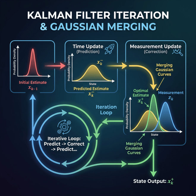
That sounds similar to a Kalman filter, and it is. Both methods are used for filtering. Both methods combine a model of how the system evolves with noisy observations of that system. Both methods are trying to answer the same basic question:

Given everything I have observed so far, what do I believe about the current hidden state?

The difference is how belief is represented.

A Kalman filter represents belief with a Gaussian distribution. In practice, this means it keeps track of a mean and covariance.

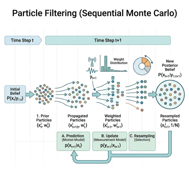
A particle filter represents belief with many weighted samples. These samples are called particles.

Each particle is one possible version of the hidden state. The weight attached to that particle tells us how plausible that possible state is.

{x_t^k, w_t^k}_k=1^K

Here, x_t^k is the k-th particle at time t, w_t^k is its weight, and K is the total number of particles.

NOTE: A particle is just a sampled hypothesis about the hidden state. A cloud of weighted particles is an approximation to a probability distribution.

What Is a Particle Filter Used For?

Particle filters are used when we need to estimate a hidden state over time, but the uncertainty is too complicated for a simple Gaussian approximation.

They are common in robotics, object tracking, target localization, navigation, nonlinear time-series analysis, ecological modeling, econometrics, signal processing, and fault detection.

A classic example is robot localization.

Suppose a robot is moving through a building. The robot has a map, but it does not know exactly where it is. Its sensors are noisy. Several hallways may look similar. Several locations may explain the same observation.

A particle filter can keep multiple possible robot locations alive at the same time.

Some particles may represent the robot being in hallway A.
Some particles may represent the robot being in hallway B.
Some particles may represent the robot being in a nearby room.

As new observations arrive, the particle filter gives more weight to the particles that better explain the data.

This is the main advantage of particle filters: they do not have to compress uncertainty into one Gaussian blob.

What Problems Are Particle Filters Good For?

Particle filters are useful when uncertainty is complicated.

They are especially good for problems with nonlinear dynamics, nonlinear observations, non-Gaussian noise, ambiguous measurements, multiple possible explanations, tracking under occlusion, sudden changes, or regime switches.

The key idea is that a particle filter can represent a distribution with many shapes.

It can represent skewed uncertainty. It can represent heavy-tailed uncertainty. It can represent uncertainty with several separate modes.

For example, if an object disappears behind another object in a video, there may be several plausible places where it could reappear. A particle filter can keep particles in several of those plausible places until the next observation makes the situation clearer.

A Simple Example: Robot Localization

Suppose a robot is trying to localize itself inside a building.

The hidden state is the robot’s position and orientation.

x_t = [x-position_t, y-position_t, orientation_t]

The robot receives sensor measurements. These might be distances to walls, visual features from a camera, or laser range measurements.

The observation at time t is:

y_t = sensor measurement at time t

At the beginning, the robot may not know where it is. So we initialize many particles across the map.

Each particle is one guess about the robot’s pose.

One particle might say: maybe the robot is in this hallway, facing north.

Another particle might say: maybe the robot is in that room, facing east.

Another particle might say: maybe the robot is near this wall, facing south.

Now the robot moves.

Each particle is moved forward according to the motion model.

x_t^k ~ p(x_t | x_t-1^k)

This means that the k-th particle at time t is sampled from the transition model, given where that particle was at the previous time step.

In plain language:

Move each possible robot pose forward according to the robot’s motion model, but include motion noise.

Then the robot receives a new sensor measurement.

For each particle, we ask:

If the robot were actually at this particle’s location, how likely would this sensor measurement be?

Particles that explain the measurement well receive high weights. Particles that explain the measurement poorly receive low weights.

w_t^k ∝ p(y_t | x_t^k)

This says that the weight of particle k is proportional to the likelihood of the observation under that particle.

After computing the weights, we normalize them so they sum to one.

w_t^k = w_t^k / Σ_j=1^K w_t^j

Now the normalized weights can be treated like probabilities over particles.

The Particle Filter Algorithm

The basic particle filter has three main steps.

Propagate the particles through the motion model.
Weight the particles using the new observation.
Resample the particles so that plausible particles survive.

Then repeat.

This is why particle filters are also called Sequential Monte Carlo methods.

“Monte Carlo” means we approximate distributions using samples.

“Sequential” means we update those samples over time as new observations arrive.

Resampling

After a few time steps, many particles may have weights close to zero. Only a few particles may explain the observations well.

This is called particle degeneracy.

Degeneracy means we are wasting computation on particles that no longer matter.

To fix this, particle filters usually resample.

During resampling, high-weight particles are likely to be copied. Low-weight particles are likely to disappear.

Suppose four particles have normalized weights:

[0.05, 0.45, 0.40, 0.10]

The second and third particles are much more likely to survive than the first and fourth particles.

After resampling, we still have the same number of particles, but more of them are concentrated in plausible regions of the state space.

NOTE: Resampling is useful, but it can also reduce diversity. If we keep copying the same high-weight particles, the particle population may lose alternative explanations too quickly.

What Is Required to Set Up a Particle Filter?

To use a particle filter, we need more than just particles. We need to define the probabilistic model that tells the particles how to move, how to compare themselves to data, and how to survive over time.

A particle filter needs five main ingredients.

A hidden state. This is what we are trying to estimate.
A transition model. This tells us how the hidden state evolves from one time step to the next.
An observation model. This tells us how likely an observation is, given a possible hidden state.
An initial particle distribution. This tells us where the particles should start.
A resampling rule. This tells us when and how to copy high-weight particles and remove low-weight particles.

The most important modeling choice is the hidden state.

If the state is too small, the filter will not contain enough information to predict the future. If the state is too large, the filter may need an enormous number of particles to work well.

For a robot, the state might be position and orientation:

x_t = [x-position_t, y-position_t, orientation_t]

For an object in a video, the state might include position, velocity, width, and height.

For a biological or medical time-series problem, the state might include an unobserved disease burden, a latent response level, or a patient-specific trajectory variable.

The key question is:

What information does the filter need to carry forward so that it can explain future observations?

How to Build the Particle Filter

Once the hidden state is defined, the next step is to define the transition model.

The transition model answers:

If the system is currently in this state, where could it plausibly go next?

In notation, we write this as:

x_t ~ p(x_t | x_t-1)

This means the next state is sampled from a distribution that depends on the previous state.

For a robot, this might use a motion model. If the robot moves forward, each particle moves forward too, but with some noise. That noise matters because real movement is imperfect.

After defining the transition model, we define the observation model.

The observation model answers:

If this particle were the true state, how likely would the observed data be?

This is the likelihood:

w_t^k ∝ p(y_t | x_t^k)

This is where the data enters the filter. A particle survives because it predicts observations that look like the observations we actually received.

Then we normalize the weights, resample particles, and repeat the process at the next time step.

In practice, the workflow looks like this:

Choose the hidden state.
Initialize many particles.
Move each particle forward using the transition model.
Compare each particle to the new observation.
Assign a weight to each particle.
Normalize the weights.
Resample if the particle population has degenerated.
Use the resulting particles to estimate the current state.

For example, the current state estimate might be the weighted average of the particles, but that is not always the only useful summary. Sometimes the full particle cloud is more informative than a single average.

NOTE: If the posterior has two modes, the weighted average may fall between them and may not represent a realistic state. In that case, it is better to inspect the particle distribution itself.

What to Look For

When a particle filter is working well, the particles should behave in a sensible way.

Early on, the particles may be spread out because uncertainty is high. As observations arrive, particles should begin concentrating in regions that explain the data well.

Good signs include:

particles concentrate around plausible states,
high-weight particles are consistent with observations,
the filter does not collapse too early,
multiple hypotheses survive when the data are genuinely ambiguous,
uncertainty decreases when observations are informative,
uncertainty increases when observations are missing or noisy.

The particle cloud should tell a story. If the data are clear, the particles should agree. If the data are ambiguous, the particles should preserve that ambiguity instead of pretending to be certain.

What to Watch Out For

Particle filters are flexible, but they can fail in predictable ways.

The first problem is particle degeneracy.

This happens when almost all particles have tiny weights and only a few particles carry most of the probability mass.

A common diagnostic is the effective sample size. It estimates how many particles are actually contributing.

ESS = 1 / Σ_k=1^K (w_t^k)²

If the effective sample size is low, the filter is relying on too few particles. That usually means resampling is needed.

The second problem is particle impoverishment.

This happens after resampling, when many particles become copies of the same high-weight particles. The filter may look confident, but it has lost diversity.

This can be dangerous because the filter may commit too early to one explanation and lose other plausible hypotheses.

The third problem is a poor transition model.

If the transition model does not allow particles to move into the region where the true state is, then the filter cannot recover. No amount of weighting can save particles that never reach plausible states.

The fourth problem is a poor observation model.

If the likelihood is too sharp, the filter may kill off too many particles. If the likelihood is too broad, the observations may not influence the particles enough.

The fifth problem is too few particles.

Particle filters can struggle in high-dimensional spaces because the number of particles needed may grow very quickly. This is one reason particle filters are powerful but not magical.

In practice, you should watch for these warning signs:

one particle receives almost all the weight,
particles collapse into a tiny region too early,
particles remain spread out even after informative observations,
the filter is very sensitive to random seed,
state estimates jump erratically,
the weighted average gives an impossible or meaningless state.

When these happen, the issue is usually not just the particle filter algorithm. It is often the model setup: the state definition, transition model, observation model, noise assumptions, or number of particles.

A Practical Way to Think About It

A particle filter is not just a computational trick. It is a way of carrying uncertainty through time.

To set it up well, think like this:

What are the possible states of the world?

How can those states evolve?

What observations would each state produce?

Which possible states should survive after seeing the data?

That is the whole logic of the particle filter.

The particles represent possible states. The transition model moves them forward. The observation model scores them. Resampling reallocates computation toward the states that remain plausible.

If those pieces are well designed, the filter can represent complicated uncertainty in a way that a single Gaussian belief cannot.

The Bayesian View

The goal of filtering is to estimate:

p(x_t | y₁, …, y_t)

This is the distribution of the current hidden state, given all observations so far.

A Kalman filter solves this exactly when the model is linear and Gaussian.

A particle filter approximates this distribution using weighted particles.

p(x_t | y₁, …, y_t) ≈ Σ_k=1^K w_t^k δ(x_t − x_t^k)

This notation says that the posterior distribution is approximated by point masses at the particles, weighted by their normalized weights.

The symbol δ represents a point mass. In plain language, it places probability directly on a particle.

You do not need to love this notation to understand the idea.

The posterior is represented by many weighted guesses instead of by one Gaussian distribution.

Discussion

Particle filters are powerful because they can keep multiple hypotheses alive.

This matters when observations are ambiguous.

Suppose a robot could be in two similar-looking rooms. A Kalman filter may average those two possible locations and place the robot somewhere between them. A particle filter can place some particles in one room and some particles in the other room.

Then, as more observations arrive, the particles in the better location receive higher weights and survive.

So the particle filter does not have to decide too early.

That flexibility is the main advantage.

But flexibility has a cost.

Particle filters can be computationally expensive. If the state space is high-dimensional, we may need many particles to approximate the posterior well.

If we use too few particles, the filter can collapse onto a small number of states. Resampling helps with degeneracy, but it can also reduce diversity.

So particle filters are not automatically better than Kalman filters.

A Kalman filter is usually better when the system is approximately linear, Gaussian, and real-time efficiency matters.

A particle filter is usually better when the posterior is nonlinear, non-Gaussian, multimodal, or ambiguous.

The simplest summary is:

A Kalman filter tracks one Gaussian belief over time.

A particle filter tracks many possible states over time.

Both are Bayesian filters.

They differ mainly in how they represent uncertainty.

Kalman Filter

A Kalman filter is a method for estimating the hidden state of a system as that system changes over time.

That sounds abstract, so let’s make it concrete.

Suppose we are tracking something that moves: a drone, a robot, a car, a satellite, or even a signal in a sensor. The object has a true state, but we do not get to observe that state perfectly.

For example, a drone has a true position and velocity. But our sensor may only give us a noisy measurement of position.

So we have two things:

1. The real state of the system.

2. A noisy observation of that state.

The job of the Kalman filter is to combine these two pieces of information over time.

It asks:

Given what I believed before, and given the noisy measurement I just received, what should I believe now?

This is the basic filtering problem.

What Is a Kalman Filter Used For?

Kalman filters are used for real-time state estimation.

They are common in navigation, robotics, aerospace engineering, control systems, computer vision, economics, and signal processing.

A classic example is GPS tracking.

GPS measurements are noisy. If you look at raw GPS data, the estimated position may jump around even when the object is moving smoothly. A Kalman filter can smooth those measurements by combining them with a motion model.

The motion model says something like:

If the object was here before, and it was moving with this velocity, then it should probably be over here now.

The measurement says:

The sensor thinks the object is here.

The Kalman filter combines both.

It does not blindly trust the model.
It does not blindly trust the sensor.
It balances them according to their uncertainty.

What Problems Are Kalman Filters Good For?

Kalman filters are especially good for problems where the system is approximately linear and the noise is approximately Gaussian.

In simple terms, this means:

the system evolves in a fairly smooth way,
measurements are noisy but not wildly unpredictable,
uncertainty can be reasonably represented by a bell-shaped distribution.

The Kalman filter represents belief using two things:

a mean,
a covariance.

The mean is the best estimate of the hidden state.

The covariance describes how uncertain we are about that estimate.

So instead of storing every possible state the system could be in, the Kalman filter stores a compact summary of belief.

That is why it is so efficient.

A Simple Example

Suppose we are tracking a drone moving in one dimension.

The hidden state contains position and velocity.

x_t = [position_t, velocity_t]

The sensor only measures position, and the measurement is noisy.

y_t = \text{noisy position measurement}

At time t-1, suppose the drone is estimated to be at position 10 and moving with velocity 2.

Before seeing the next measurement, the model predicts that the drone should be near position 12.

That is the prediction step.

Then the sensor reports position 13.5.

Now we have a disagreement.

The model says: I expected the drone near 12.

The sensor says: I measured the drone near 13.5.

The Kalman filter combines these two pieces of information.

If the sensor is very reliable, the updated estimate moves closer to 13.5.

If the sensor is noisy, the updated estimate stays closer to 12.

This balance is controlled by the Kalman gain.

The Kalman gain determines how much the filter trusts the new measurement compared to the model prediction.

The Model

A standard Kalman filter assumes a linear state-space model.

The state evolves like this:

x_t = A x_{t-1} + error

The observation is generated like this:

y_t = C x_t + error

The first equation says that the current state depends on the previous state.

The second equation says that the observation is a noisy measurement of the current state.

Here, A describes the system dynamics. For example, it tells us how position and velocity change over time.

The matrix C describes what part of the hidden state we actually observe.

NOTE: We may care about both position and velocity, but only measure position directly. The velocity still matters because it helps predict future position.

The Bayesian View

The Kalman filter is a Bayesian filter.

That means it keeps updating a probability distribution over the hidden state as new observations arrive.

The object we want is the filtering distribution:

p(x_t | y_1, …, y_t)

This means: the probability distribution of the current hidden state, given all observations so far.

The Kalman filter is special because, under linear Gaussian assumptions, this distribution stays Gaussian.

So the filter does not need to store a complicated distribution.

It only stores the mean and covariance.

That is the entire reason the Kalman filter is so clean.

Discussion

The Kalman filter is powerful because it is fast, elegant, and interpretable.

It is fast because it only updates a mean and covariance.

It is elegant because it gives the exact Bayesian filtering solution when the model is linear and Gaussian.

It is interpretable because the uncertainty has a clear meaning. If the covariance is large, the filter is uncertain. If the covariance is small, the filter is confident.

But the Kalman filter also has limitations.

The main limitation is that it represents uncertainty as one Gaussian distribution.

That is fine when the uncertainty has one main center.

But suppose a robot is in a building and there are two hallways that look almost identical. The robot may plausibly be in hallway A or hallway B.

That belief has two modes.

A Kalman filter may average those two possibilities and put the robot somewhere between the hallways, possibly inside a wall.

That is not just a bad estimate. It is a bad representation of uncertainty.

So the Kalman filter works best when one Gaussian belief is a reasonable approximation.

When the posterior distribution is nonlinear, non-Gaussian, or multimodal, we often need something more flexible.

That leads us to particle filters.

How to Think Through a Kalman Filter Problem

When setting up a Kalman filter, the hardest part is usually not the algebra. The hardest part is deciding what the hidden state should be and how the measurements relate to that state.

A good way to think through the problem is to ask four questions.

First:

What am I trying to estimate?

This determines the hidden state ( $x_t$ ).

For the drone example, we may want to estimate both position and velocity:

x_t = \begin{bmatrix} \text{position}_t \ \text{velocity}_t \end{bmatrix}

Even if we only measure position, velocity is still useful because it helps us predict future position.

Second:

How does the state evolve from one time step to the next?

This determines the transition model.

For a simple constant-velocity model, position changes according to velocity. If the time step is ( $\Delta t$ ), then:

\text{position} t = \text{position}{t-1} + \Delta t \cdot \text{velocity}_{t-1}

and velocity may stay approximately the same:

\text{velocity}t = \text{velocity}{t-1}

In matrix form, this becomes:

x_t = A x_{t-1} + \epsilon_t

where (A) is the state-transition matrix and ( $\epsilon_t$ ) is process noise.

For this constant-velocity example, the transition matrix is:

A = \begin{bmatrix} 1 &amp; \Delta t \ 0 &amp; 1 \end{bmatrix}

This matrix says:

new position equals old position plus velocity times time,
new velocity equals old velocity.

Third:

What do I actually observe?

This determines the observation model.

If the sensor only measures position, then the observation is:

y_t = \text{noisy position measurement}

In matrix form:

y_t = C x_t + \delta_t

where (C) selects the part of the hidden state that the sensor can observe.

For position-only measurements,

C = \begin{bmatrix} 1 &amp; 0 \end{bmatrix}

This means:

observe position, but do not directly observe velocity.

Fourth:

How noisy are the model and the measurements?

This determines the covariance matrices.

The process-noise covariance (Q) describes uncertainty in the dynamics. It answers:

How much do I trust my motion model?

The measurement-noise covariance (R) describes uncertainty in the sensor. It answers:

How much do I trust my observations?

If (R) is large, the measurements are noisy, so the filter trusts the model more.

If (R) is small, the measurements are reliable, so the filter trusts the observations more.

If (Q) is large, the model dynamics are uncertain, so the filter is more willing to adjust when new measurements arrive.

If (Q) is small, the model is trusted more strongly.

NOTE: Choosing (Q) and (R) is one of the most important practical parts of using a Kalman filter. The equations may be correct, but poor noise assumptions can make the filter behave badly.

What Is Required?

To run a Kalman filter, we need five main ingredients.

An initial state estimate.

\mu_0

This is our best guess of the starting state.

An initial uncertainty estimate.

\Sigma_0

This says how uncertain we are about the initial state.

A transition model.

A

This describes how the state evolves.

An observation model.

C

This describes how the hidden state produces measurements.

Noise covariances.

Q \quad \text{and} \quad R

The matrix (Q) describes process noise.
The matrix (R) describes measurement noise.

Once these are specified, the Kalman filter can run recursively.

How the Solution Proceeds

At each time step, the Kalman filter performs two operations: prediction and update.

The prediction step asks:

Before seeing the new measurement, where do I expect the state to be?

The predicted mean is:

\mu_{t|t-1} = A\mu_{t-1}

The predicted covariance is:

\Sigma_{t|t-1} = A\Sigma_{t-1}A^T + Q

The update step asks:

After seeing the new measurement, how should I revise my belief?

First, compute the innovation:

r_t = y_t – C\mu_{t|t-1}

The innovation is the difference between what we observed and what the model expected us to observe.

Then compute the innovation covariance:

S_t = C\Sigma_{t|t-1}C^T + R

This describes how uncertain we are about the innovation.

Then compute the Kalman gain:

K_t = \Sigma_{t|t-1}C^T S_t^{-1}

The Kalman gain determines how strongly the new measurement should change the estimate.

Finally, update the mean and covariance:

\mu_t = \mu_{t|t-1} + K_t r_t

\Sigma_t = (I – K_t C)\Sigma_{t|t-1}

Then the filter moves to the next time step and repeats the same process.

The Practical Recipe

So the practical recipe is:

Define the hidden state.
Define how the state evolves.
Define what the sensor observes.
Estimate the process noise (Q).
Estimate the measurement noise (R).
Initialize the state mean and covariance.
Repeat prediction and update as new measurements arrive.

This is why the Kalman filter is so useful.

Once the problem is written as a state-space model, the filtering procedure is automatic.

The real modeling work is deciding what belongs in the state, how the state evolves, what the observations measure, and how much uncertainty belongs in the model and the sensor.