Sequential Monte Carlo (SMC)

June 10, 2019
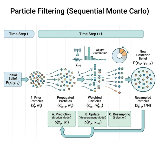
We begin with a short recap of all the previous algorithms we discussed that are prerequisite to Sequential Monte Carlo. Then I intuitively describe how SMC works. After, we dig into the math behind SMC. We first discuss how importance weights are calculated at each time step, and then we discuss how SMC maintains this notion of survival of the fittest with sample trajectories through resampling.

Before we start, I’d like to thank Jan-Willem van de Meent for his lectures in his Advance Machine Learning Class for PhD students at Northeastern University. The images shown are inspired by his lectures. In addition, I’d like to address that more details on SMC can be found in An Introduction to Probabilistic Programming available [arXiv]. This book is intended as a graduate-level introduction to probabilistic programming languages and methods for inference in probabilistic programs.

Mini Review

Before we move on to other Monte Carlo estimators we might use in machine learning, let’s recap:
- We have discussed what a Monte Carlo Estimator is. It helps us estimate an expectation of some function via sampling.
- We introduce Importance Sampling as our first Monte Carlo Estimator. We learn that Importance Sampling requires us to evaluate samples using a normalized density, which is something we cannot do (almost always).
- Then we describe Self-Normalized Importance Sampling (SNIS). SNIS uses two Monte Carlo Estimators; the same one in Importance Sampling and a second one to estimate the normalization constant. This allows us to evaluate samples via an unnormalized density, which we have access to.
- Importance Sampling methods give us marginal likelihoods, but the downfall is that they do random guessing.
- We then discuss Monte Carlo Markov Chains (MCMC). MCMC uses transition kernels that let us stay in the target density once we have a good sample (one from the target density). However, (almost always) successful MCMC algorithms need to satisfy detailed balance.
- We learn that Metropolis-Hastings (a fancy MCMC algorithm) let’s us use any proposal due to an acceptance probability it uses to manage detailed balance for us.
- In the previous post, we describe an algorithm that marries Importance Sampling and MCMC, Annealing Importance Sampling. This algorithm successfully breaks a hard problem into a series of simpler problems. It provides a marginal likelihood and uses a transition kernel.
Now we will introduce another Monte Carlo Estimator that is used for a set of different problems in machine learning, Sequential Monte Carlo.

Tick Tock: Introducing Time to the Problem!

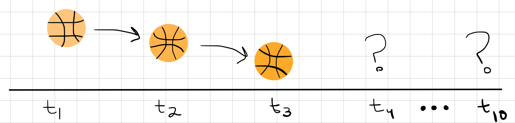
All of the algorithms we have discuss so far are for problems for which we do not need to consider the element of time! What does that mean? Let’s consider an example of looking at a sequence of video frames of a basketball moving from time frame to time frame.

We record that at time $t_1$ (which can be any arbitrary time stamp), the ball to be up high. We continue to watch the ball move at $t_2$ and $t_3$ , steadily moving downward. The question we have is, “Where will the ball be in the future? This time-dependent data is referred to as time-series data.

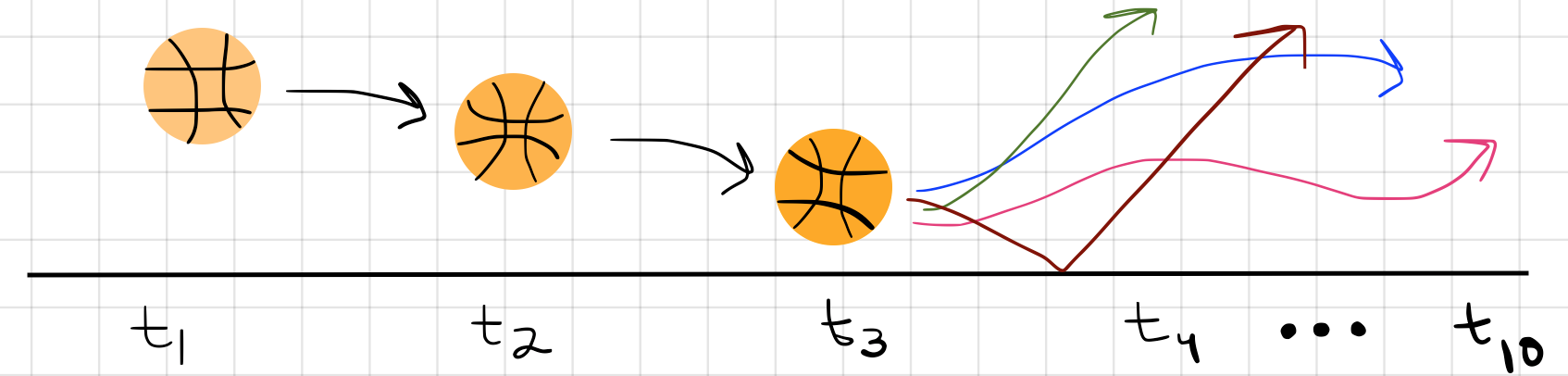
There are many combinations of future movements the ball can make. Several can make sense by following the laws of physics, others can be absolutely garbage (like the ball suddenly shooting upwards, or spelling out a word).

Now consider using any of the Monte Carlo Estimating algorithms we have already discussed. If our data is time dependent, then Importance Sampling would have a very difficult time picking up a pattern that correlates movements between frames. It would probably take ages to get a good set of samples from the posterior! Instead, we can use a more appropriate algorithm for time-dependent problems, such as Sequential Monte Carlo (SMC).

Intuition behind Sequential Monte Carlo

SAMPLING BUDGET. Let’s start off by stating that every sampling scheme has this notion of a sampling budget. This sampling budget (or sample budget) is the maximum number of samples we can afford to use. The number in our budget may depend on the computer we use, the dimensionality of the problem, or even just the amount of time we can afford running our algorithm (because these algorithms do take time!). Usually we use the notation $S$ to represent the number of samples in our sample budget, $x^1, x^2, ... x^S$ .

In time-series problems, we perform inference (using some form of Monte Carlo Estimator) at each time step. This means we use the same number of samples for each time step, i.e. the number of samples in our sampling budget, $S$ .

NOTE: People have adopted the term particle to replace the term sample. Instead of saying we have a sampling budget of 10 samples… it’s common to say we have a sampling budget of 10 particles.

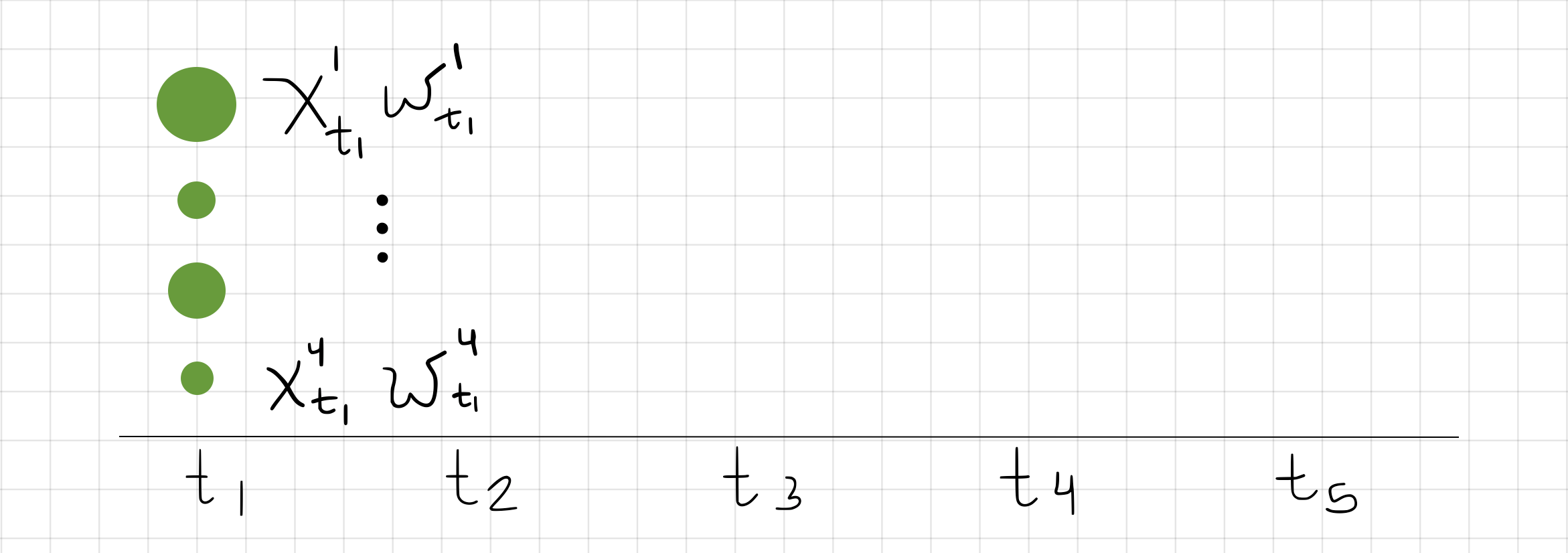
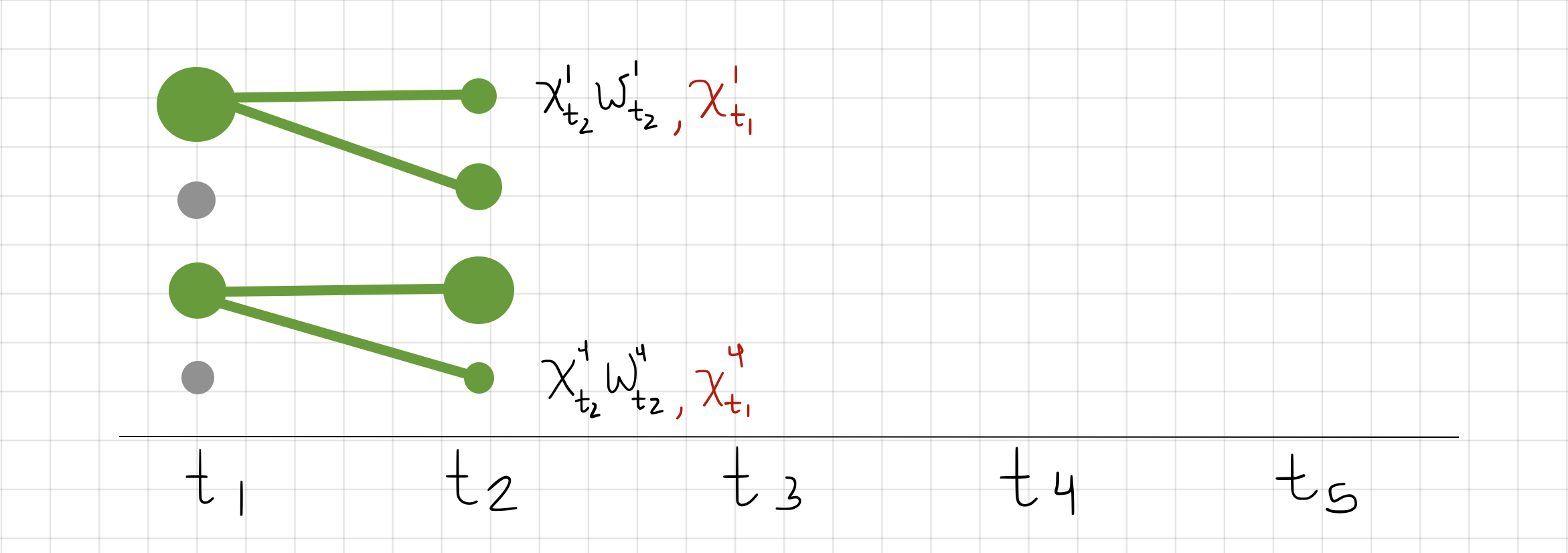
So let’s now consider an example where we have a sampling budget of four, $S= 4$ , and we are working with a small problem with five time steps, $t_1, ... t_5$ . Imagine that each sample represents the position of the ball at its respective time frame. Below we show an example where we have 4 samples at $t_1$ , represented by circles, $x^1, x^2, ..., x^4$ . You can image that these samples represent 4 guesses of the position of the ball for the data from the video frame. Now imagine that each sample (or ball position) has an associated importance weight (just like we discussed in Importance Sampling), $(x^1, w^1), (x^2, w^2), ..., (x^4, w^4)$ . The weight tells us how well the ball position matches the data in the video frame. In the figure below, I drew larger circles to represent higher importance weights and smaller circles to represent lower importance weights.

So what SMC does next is decide which samples we should keep and which ones which throw away. This is a way of saying that some guesses of the ball’s position are going to be good ones, and some will be not so good. We want to keep working with our already good guesses at the next time step, so that we can build on those guesses with other guesses. We do this by resampling. This means we will sample with replacement 4 new samples to build on in the next time step, $t_2$ . We resample based by their weights (we’ll go more into detail in a bit).

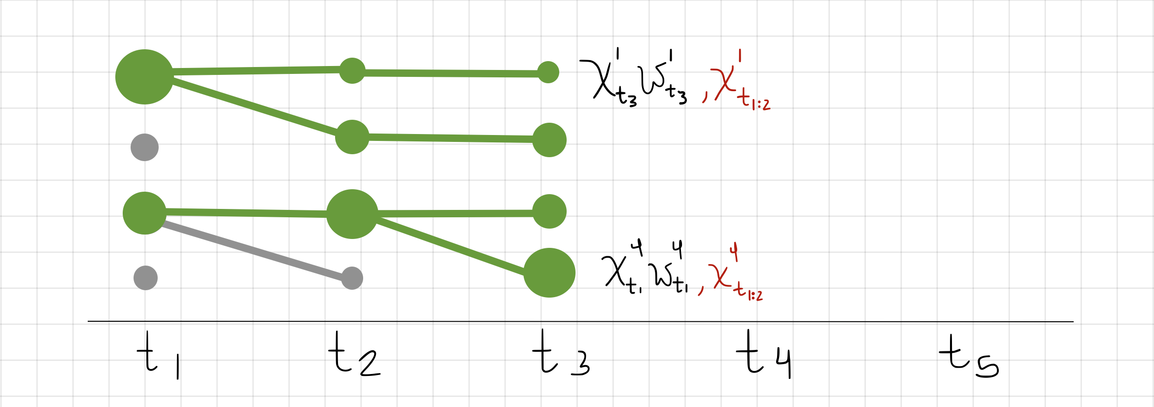
In the figure above, it so happened that we resampled $x^1_{t_1}$ twice and $x^3_{t_1}$ again, twice. This means that those samples for the ball’s position were really good, and we want to keep working with those samples. Now at $t_2$ , we sample new ball positions for that time step, $(x^s_{t_2}, w^s_{t_2})$ , but keep into account the ball positions we resampled from the past (red notation above, $x^{s}_{t_1}$ ).

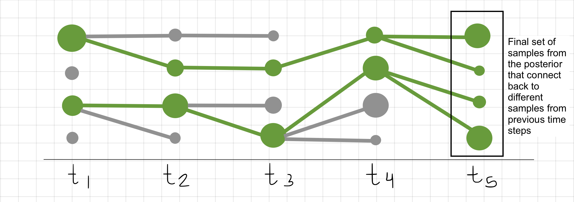
If we move on to $t_3$ , we start to notice how certain trajectories (such as the one in gray) start dying out. This means that some sequences of ball positions will NOT be used for at future time steps.

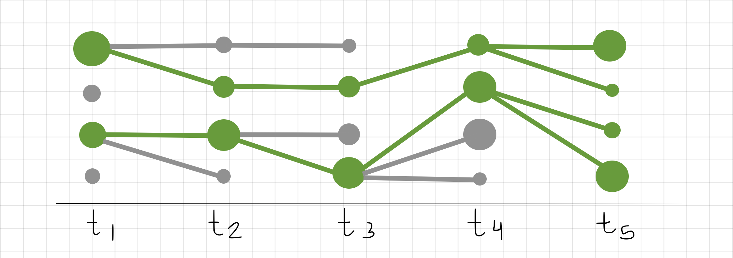
We can continue this pattern until we reach the last time step, $t_5$ . We will see that by then we still have 4 samples. However these 4 samples represent full trajectories, $x^{1}_{t=1:5}, ... , x^4_{t=1:5}$ ; these samples connect back to previous time steps. Full trajectories represent entire sequences of ball movements. The ones that survived are the ones that best match our video frame data.

Now that we have described how SMC behaves, let’s be a bit more precise and dig into the math. Don’t worry, I’ll explain it as I use it.

Math Behind Sequential Monte Carlo

Let’s break this discussion into 2 parts. We’ll first discuss the Importance Sampling bit of SMC, and then we’ll discuss Importance Resampling.

Idea 1: Sequential Importance Sampling

As we previously mentioned, our samples have an associated importance weight. In a Monte Carlo estimate, an importance weight of a sample is evaluated in the same pattern we have seen before, with some unnormalized density and the proposal, $w =\frac{\gamma(x)}{q(x)}.$

Since we are now working with time-series data, we are working with a sequence of samples. Remember that with any problem we have data we observe, $y$ , and data we are trying to learn, $x$ (sometimes referred to as states, or hypothesis). In the example above, $y$ would be the video frame data and $x$ would be the positions of the ball that we are trying to learn/predict.

So in Sequential Monte Carlo, our importance weight really looks more like this:

$w_t = \frac{p(y_{1:t}, x_{1:t})}{q(x_{1:t})}$

where $p(y_{1:t}, x_{1:t})$ represents our unnormalized density and $q(x_{1:t})$ is our proposal. These two distributions take time into consideration; meaning that the densities account for all the samples at each time step.

NOTE: $p(y_{1:t}, x_{1:t})$ is equivalent to $p(y_1, y_2, ...., y_t, x_1, x_2, ..., x_t)$

Let’s expand our unnormalized density using the chain rule:

$p(y_{1:t}, x_{1:t}) = p(y_{t}, x_{t} \mid x_{1:t-1}) p(y_{1:t-1}, x_{1:t-1})$

This is a way of expressing the density that predicts the $t^{th}$ video frame and ball position given the previous $1 : (t-1)$ video frames and ball positions.

And let’s do the same for our proposal distribution:

$q(x_{1:t}) = q(x_{t} \mid x_{1:t-1}) q(x_{1:t-1})$

Now that we have these two expanded forms of the distribution, let’s see how they look as an importance weight.

$w = \frac {p(y_{t}, x_{t} \mid x_{1:t-1}) } { q(x_{t} \mid x_{1:t-1})} \frac{p(y_{1:t-1}, x_{1:t-1})}{ q(x_{1:t-1})}$

This looks kind of messy. Let’s clean it up a bit. Remember that using chain rule, we could expand our unnormalized density as $p(y_{1:t}, x_{1:t}) = p(y_{t}, x_{t} \mid x_{1:t-1}) p(y_{1:t-1}, x_{1:t-1})$ . Notice how we can solve for $p(y_{t}, x_{t} \mid x_{1:t-1})$ :

$p(y_t, x_t|x_{1:t-1}) = \frac{p(y_{1:t}, x_{1:t})}{p(y_{1:t-1}, x_{1:t-1})}$

If we replace $p(y_t, x_t|x_{1:t-1})$ in the importance weight with the fraction above:

$w_t = \frac {p(y_{1:t}, x_{1:t}) } { p(y_{1:t-1}, x_{1:t-1}) q(x_{t} \mid x_{1:t-1})} \frac{p(y_{1:t-1}, x_{1:t-1})}{ q(x_{1:t-1})}$

we can recognized that the second fraction is an importance weight for the previous time step:

$w_{t-1} = \frac{p(y_{1:t-1}, x_{1:t-1})}{ q(x_{1:t-1})}$

which means our sequential importance weights are updated from time step to time step based on previous weights:

$w_t = \frac {p(y_{1:t}, x_{1:t}) } { p(y_{1:t-1}, x_{1:t-1}) q(x_{t} \mid x_{1:t-1})} \frac{p(y_{1:t-1}, x_{1:t-1})}{ q(x_{1:t-1})}$
$= \frac {p(y_{1:t}, x_{1:t}) } { p(y_{1:t-1}, x_{1:t-1}) q(x_{t} \mid x_{1:t-1})} w_{t-1}$

We can generalize using unnormalized densities if we say:

$p(x_t, y_t|x_{1:t-1}) = \frac{p(x_{1:t}, y_{1:t})}{p(x_{1:t-1}, y_{1:t-1})} = \frac{\gamma_t(x_{1:t})}{\gamma_{t-1}(x_{1:t-1})}$

Which means we can formulate a generalized update of importance weights at each next time step:

$w_t = \frac {\gamma_t(x_{1:t})} { \gamma_{t-1}(x_{1:t-1})q(x_{t} \mid x_{1:t-1})} w_{t-1}$

And there you have it! This is how we do the importance sampling in sequential problems. The importance weight of current samples depend on the importance weights of previous samples.

Idea 2: Importance Resampling

If we refer back to the intuition behind SMC, you’ll remember that we pick which sequence of samples we decide to reuse for future sampling.

When we decide that a sequence of samples no longer matches our observations well enough, or aren’t strong enough explanations of the data as other sequences of samples, we stop using them (refer to grey sequences in the figure above). These sequences die out because they were not chosen to continue based on their importance weights. We can think of this process as natural selection. The best sequences will continue to the end, while others will die out on their journey to the end.

Remember that at each time step, we work with a sample budget. We’re going to change notation a bit and now say that we have a sample budget of $K$ samples. So in SMC, at each time step, we sample $K$ particles, and compute an importance weight for each.

$w^k = \frac{\gamma(x^k)}{q(x^k)} \qquad x^k \sim q(x^k) \qquad k = 1, ..., K$

At this point, all of the particles’ importance weights are unnormalized. This means that they do not sum to 1. So in order to choose which samples are more fit than others (i.e. have proportionally higher weights), we normalize the importance weights.

$\bar{w^k} = \frac{w^k}{\sum_{k'=1}^K w^{k'}}$

Now we can use these normalized weights in order to choose which ones will continue on. We do this by sampling particle indexes proportionally to their normalized weight by means of a discrete (commonly known as categorical) distribution.

$a^k \sim Discrete( \bar{w^1}, ..., \bar{w^k} ) \qquad k=1, ..., K$

$a^k$ represents a single number, 1 through $K$ , that is tells us which particle to pick. We do this K times (sample budget), and sample with replacement. This means that we can pick the same particle more than once (this usually happens with high weighted particles).

So now that we have $K$ number of numbers that are between 1 through $K$ , we pick them out!

$\tilde{x}^{k'} = x^{a^k} \qquad k'=1, ..., K \quad k=1, ..., K$

where $\tilde{x}^{k'}$ represents a fit sample that we will use for the next time step.

So far we have chosen which samples are fit, $\tilde{x}^1, ..., \tilde{x}^K$ . Our next step is to reweigh these fit samples. Since they were all chosen according to their weight, they do not sum up to 1 anymore. In fact, their weights do not fully represent their value anymore. So how do we fix this? Well, we can do this by preserving the average of the original weights, $w^1, ..., w^K$ . Let’s say that $\hat{Z}$ represents the average:

$\hat{Z} = \frac{1}{K} \sum_{k=1}^K w^k$

If we decide to set all the new weights, $\tilde w^1, ..., \tilde{w}^K$ , of all the fit samples, $\tilde{x}^1, ..., \tilde{x}^K$ to $\hat{Z}$ , then the average is the same!

$\hat{Z} = \frac{1}{K} \sum_{k=1}^K \tilde{w}^k = \frac{1}{K} \sum_{k=1}^K \hat{Z}^k$

Summary

So let’s talk about SMC some more with a sequence of question-answer pairs.
1. Why do we use SMC?
  
  We use it when we are working with time-dependent data.
2. How is SMC like previous Monte Carlo Estimators we have talked about?
  
  It’s Importance Sampling, except we update our weights with past weights, and there’s a notion of pruning out bad sequences of guesses through resampling.
3. Why do we update our weights after resampling?
  
  After resampling, we have a new collection of fit guesses/samples/particles. We do it to preserve the average of the original weights.
Thanks for reading this blog! Check out past blogs that build up to SMC.

A Tumor Graph That Forecasts Where Response May Appear, Not Only How Much

October 10, 2026

A presurgery tumor-volume estimate can be numerically close while hiding the spatial pattern that produced it. I designed this research around a stricter question: from one pretreatment dynamic contrast-enhanced breast MRI, could a model forecast how much enhancing tumor would remain, where it would remain, and how reliable the volume forecast was for that patient?

The result is a retrospective tumor-state forecasting study that combines image embeddings, an anatomy-aligned graph, and patient-conditioned conformal uncertainty. It is a research model, not a clinical decision system.

The research story in a minute

My role: I defined the longitudinal graph state, crystal-shell relations, matched controls, linked regional and volume endpoints, and uncertainty-selection protocol.
The hardest decision: A close tumor-volume estimate is not evidence that the regional pattern is correct. I tested scalar and spatial errors separately.
Evidence: The manuscript reports retrospective held-out results for 202 ACRIN-6698 patients nested in the I-SPY2 trial family, with aggregate ablations and an interval-width tradeoff.
Limit: This is not independent-trial or clinical validation. The secondary pCR classifier also uses observed early-treatment features.

Jump to: graph state and pipeline figure · regional ablation · uncertainty tradeoff · next tests and limitations.

The study at a glance

Input	One pretreatment DCE-MRI examination
State	Registered tumor supervoxels with local image, enhancement, position, and volume features
Forecaster	Frozen ResNet-18 image embeddings with crystal-shell edge-gated message passing
Primary outputs	Presurgery regional tumor state and functional tumor volume (FTV) with a patient-specific 90% interval
Evaluation	556 I-SPY2 patients for fitting and selection, then 202 held-out ACRIN-6698 patients for scoring

ACRIN-6698 is nested within the I-SPY2 trial family. The evaluation therefore measures generalization across acquisitions and sites within that trial family, not validation on an independent trial.

Why forecast a graph state?

Most response models reduce the problem to one scalar or one classification decision. A scalar FTV can describe total enhancing burden, but it cannot show whether the model placed that burden in the correct tumor regions. A pCR probability can support a response classification, but it does not expose the regional state behind the prediction.

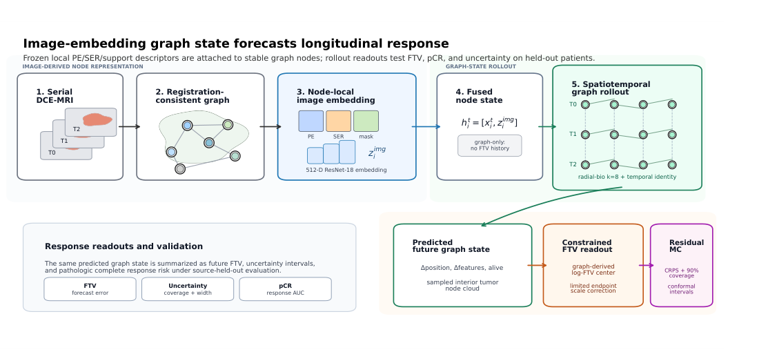
I represented the observed tumor as persistent supervoxel nodes whose identities were carried across imaging visits through registration. Each node contained local volume, position, enhancement measurements, and an embedding of the surrounding percent-enhancement and signal-enhancement-ratio patches. A frozen ResNet-18 produced those image embeddings.

The crystal-shell graph proposed connections within concentric tumor shells and across radial neighborhoods. Learned edge gates then controlled how strongly neighboring regions contributed to each update. Starting from pretreatment, the model rolled the graph state forward to presurgery. The predicted node geometry and activity produced a regional readout, while predicted node volume weighted by activity produced FTV.

Manuscript diagram showing registered image patches, persistent tumor regions, graph-state forecasting, and linked response readouts.

The frozen natural-image encoder was an experimental choice, not a claim that ImageNet pretraining is optimal for breast MRI. The important design decision was to test its contribution separately from graph communication.

Controlled comparisons explain what each component contributes

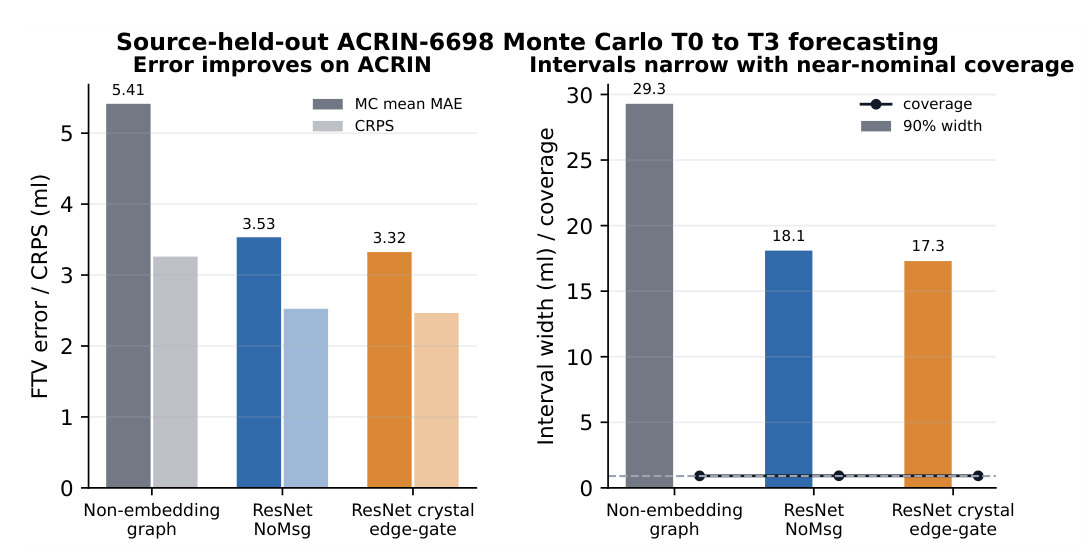
I compared three variants: a graph without image embeddings, an embedding model without neighborhood messages, and the complete image-embedding edge-gated graph. This ablation separated local image information from spatial communication.

Research question	Held-out result	Interpretation
How much tumor remained?	3.08 mL deterministic FTV MAE	The complete model recovered scalar enhancing burden at the reported error scale.
Where did it remain?	3.40 mm mean Chamfer distance	The predicted and observed enhancing point clouds were compared spatially.
Did message passing help regional prediction?	Active-region count error fell from 14.13 to 2.24	Image embeddings retained scalar accuracy, while graph communication carried much of the regional-activity signal.

The no-message model retained a similar Monte Carlo FTV point-error scale, but its regional active-subregion count error increased sharply. Restoring crystal-shell message passing reduced that error 6.3-fold, from 14.13 to 2.24, at nearly unchanged scalar accuracy. The result supports a specific interpretation of the ablation: image content predicts much of how much, while spatial communication helps predict where. It does not prove that every graph edge is biologically causal.

Aggregate held-out comparison of Monte Carlo FTV error, CRPS, interval width, and coverage across the three controlled model variants.

The 3.08 mL value is the deterministic FTV MAE. The figure above reports the separate Monte Carlo mean MAE, which was 3.32 mL for the full model.

Uncertainty must be selected without looking at the test cohort

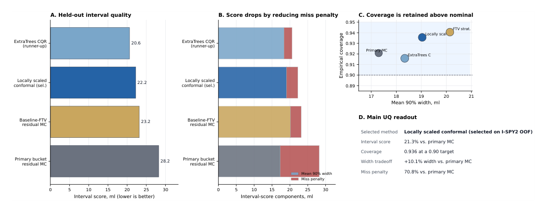
A prediction interval is useful only if its selection procedure is credible. The uncertainty pipeline first generated residual Monte Carlo FTV samples and conformal bounds. I then compared patient-conditioned recalibration methods using I-SPY2 out-of-fold interval scores under a coverage constraint. The selected locally scaled conformal method was frozen before ACRIN-6698 was scored.

On the held-out subset, the selected method changed the uncertainty readout as follows:

The 90% interval score improved from 28.24 to 22.23.
Coverage increased from 0.921 to 0.936.
Mean interval width increased from 17.30 to 19.04 mL.
The FTV point estimate did not change.

This was a useful tradeoff, not a free improvement. The interval score improved because outside-interval misses became less costly, while the average interval became wider. A different candidate achieved a lower score after ACRIN scoring, but it was not the training-selected method. Choosing it afterward would use knowledge of the held-out subset.

Held-out comparison of interval-score components, coverage, and width for the uncertainty methods.

A secondary pCR analysis needs a precise boundary

The predicted graph state also supported a secondary pathologic complete response analysis. The selected feature stack reached a held-out AUC of 0.807, while a simpler clinical-plus-graph-temporal comparator reached 0.826. These classifiers included observed early-treatment and inter-regimen features. I therefore do not describe the pCR result as a prediction from pretreatment MRI alone.

The pCR analysis tests whether the graph representation carries response-related information. It does not show that the model chooses treatment, replaces clinical interpretation, or improves patient outcomes.

What I owned as a researcher and engineer

This project required more than fitting a model. The core work was defining an inspectable longitudinal state, preserving regional identity, constructing an anatomy-aligned graph relation, designing matched controls, connecting spatial and scalar endpoints, and separating uncertainty-method selection from held-out scoring. It also required tracing every public claim back to the exact evaluation protocol and keeping the research boundary explicit.

The difficult design choice was resisting a scalar-only success criterion. FTV error is easy to summarize, but it cannot establish whether the model forecast the correct regional response. The graph-state evaluation made that failure mode visible. The uncertainty evaluation added a second discipline: coverage, width, and miss penalty had to be considered together rather than compressed into one favorable number.

What I would test next

The strongest next step is evaluation on an independent breast MRI cohort. I would also test a domain-adapted image encoder, sensitivity to incomplete visits and upstream registration failures, and whether readers use the regional forecast and interval differently from an FTV point estimate alone. A matched comparison against dedicated pCR-first models would clarify the value of the secondary classifier.

Those steps matter because this study used a selected retrospective cohort with complete imaging and successful processing. No prospective deployment or patient benefit has been demonstrated.

The contribution is a modeling framework that keeps three outputs connected: regional response, scalar tumor burden, and calibrated reliability. That combination creates a more inspectable foundation for advanced modeling than a point prediction alone, while leaving the evidence boundary intact.

Read my PhD research overview · See my production AI engineering case study · Choose a résumé

Building a Production AI Assistant for Employee Knowledge and Operations

October 9, 2026

A case study in designing a shared assistant that could answer employee questions, investigate technical problems, and take bounded action without collapsing identity, memory, and execution into one trust boundary.

An employee should not have to know which repository, handbook page, dashboard, or subject-matter expert contains the answer to a routine question. The experience I wanted was simple: ask in the team’s existing chat interface, receive a useful answer with supporting context, and continue working.

The engineering behind that experience was less simple. The assistant had to serve technical and non-technical employees, preserve individual context without mixing users, consult shared knowledge, inspect operational evidence, and occasionally run tools. It also needed to explain when the available evidence was insufficient.

I owned the production architecture around the assistant. My work centered on the service boundaries, profile and tool permissions, memory model, isolated execution path, infrastructure as code, deployment verification, observability, and recovery strategy. This case study describes that design at a level that is useful to engineers while leaving out company-specific data, internal identifiers, and security-sensitive configuration.

The engineering story in a minute

My role: I designed the production architecture around the model, including identity and memory boundaries, profile-specific tools, an isolated runner, deployment checks, and recovery.
The hardest choice: One employee interface was useful, but a single unrestricted assistant was not. I separated support and engineering capabilities behind different profiles.
What a reader can inspect: Architecture-evolution and responsibility diagrams, the request pipeline, an evaluation matrix, and the failure-to-regression process.
Evidence limit: This public account does not include employer-specific traces or performance and adoption numbers that I cannot substantiate publicly.

Jump to: architecture diagrams · the trust-boundary decision · evaluation and regression checks.

The case study at a glance

Problem: Employees needed one conversational entry point to information spread across documentation, repositories, and operational systems.
My ownership: I designed and implemented the production architecture around the model, including identity isolation, memory boundaries, tool access, sandboxed execution, deployment controls, monitoring, and recovery.
Architecture: A chat gateway routes authenticated requests into a stateful agent controller. The controller can retrieve personal context and shared knowledge, invoke bounded tools, or send technical work to an isolated runner.
Difficult design choice: I kept one employee-facing interface while separating support and engineering work into different profiles and trust boundaries.
Retrieval choice: I routed questions to different retrieval methods based on source type and authority instead of placing every source in one vector index.
Model and provider choice: I used a strong reasoning model for orchestration, smaller models for bounded supporting work, and a separate fast provider for memory operations, all behind a model gateway.
Prompt strategy: I separated stable policy, profile instructions, retrieved evidence, tool schemas, and the current request so that authority did not depend on one large prompt.
Evaluation: I tested retrieval, tool selection, privacy boundaries, abstention, long-context recovery, deployment state, and failure handling, then converted failures into regression cases.
Next-step planning: Evaluation findings become bounded engineering work with an owner, hypothesis, evidence requirement, success criterion, and regression check.
Failure strategy: The system distinguishes model uncertainty, tool denial, execution failure, deployment drift, memory failure, and infrastructure failure so that each can be handled differently.
Result: The implementation established a production foundation for a shared assistant without requiring broad access for every request. I am deliberately not attaching performance or adoption numbers that I cannot substantiate publicly.

The problem was information access, not chat

The visible request might be, “What is the current process for this issue?” A good answer could require several steps. The assistant may need to identify the employee and conversation, search a shared handbook, inspect a read-only repository, compare a current configuration with its owning code, and return a conclusion that separates observation from inference.

A single prompt could not provide those guarantees. The system needed to answer four questions before it acted:

Whose context is relevant to this request?
Which source is authoritative for the information?
Which tools is this profile allowed to use?
What evidence is required before the assistant can make a claim?

Those questions became the organizing principles for the architecture.

How the architecture evolved

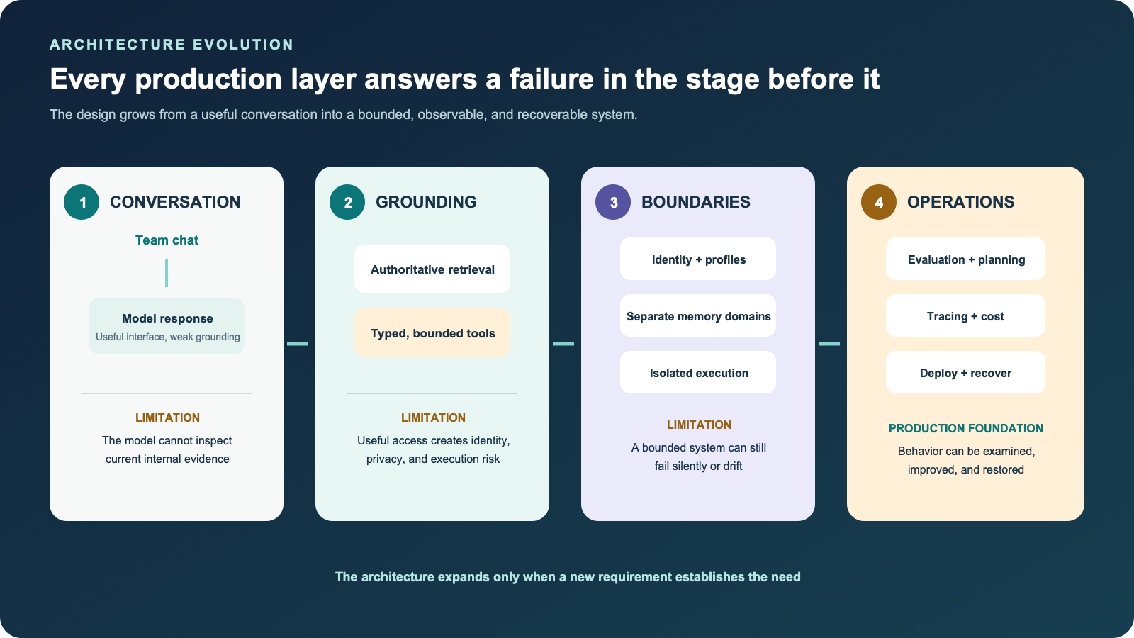
I did not begin with the final production diagram. I treated the architecture as a sequence of constraints discovered through increasingly realistic use cases.

The first stage established the employee experience: an authenticated message enters through the existing team interface and reaches a model. The second stage made the answer useful by adding authoritative retrieval and bounded tools. The third stage addressed trust by separating profiles, per-user memory, shared knowledge, and command execution. The fourth stage made the system operable through evaluation, tracing, cost attribution, immutable deployment, and recovery.

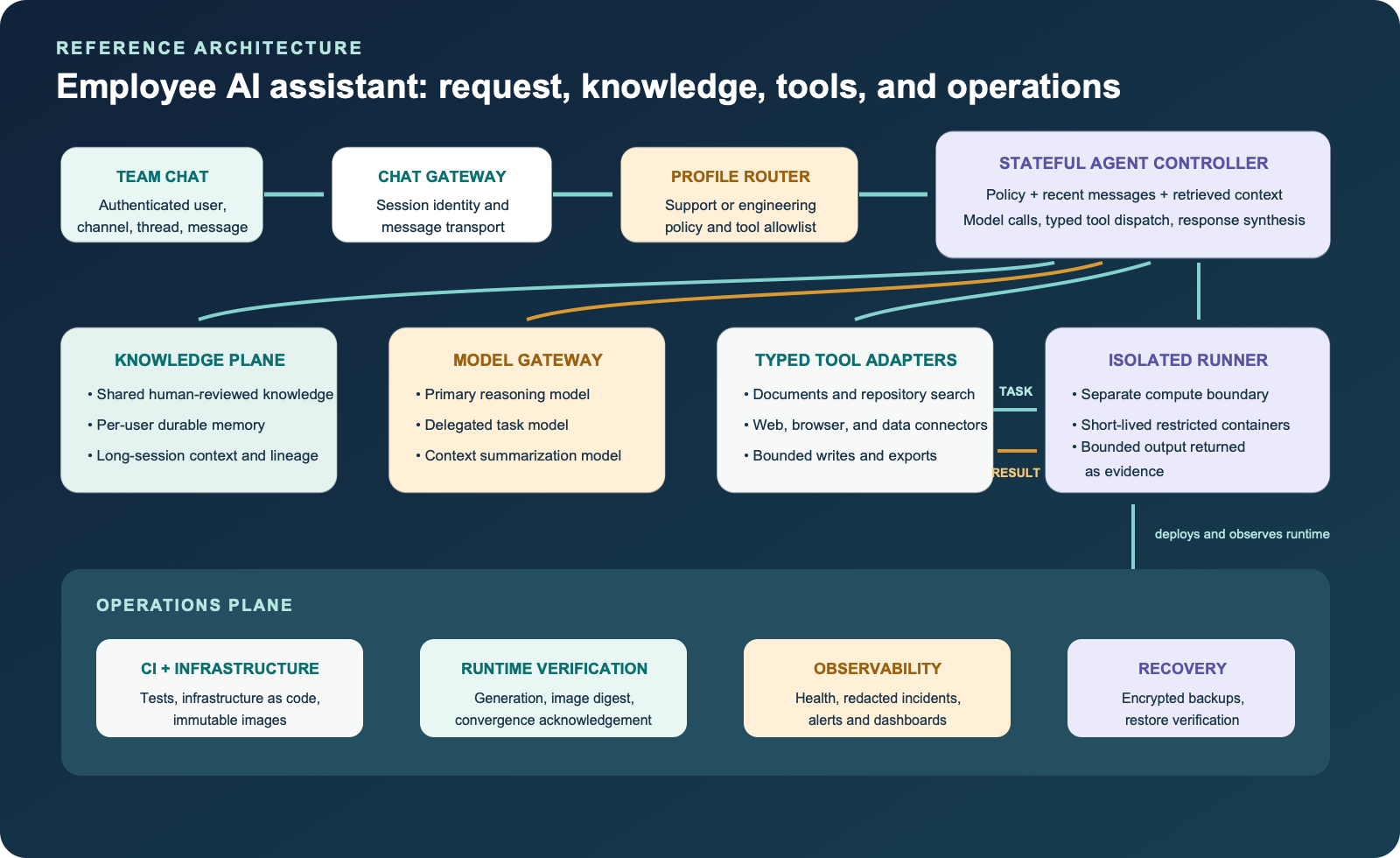
Four stages in the architecture of an employee AI assistant. The design progresses from a conversational model, to retrieval and tools, to identity and isolated execution, and finally to evaluation, observability, deployment, and recovery. — Each stage exists because the previous stage exposed a concrete limitation. The final architecture is the accumulation of those decisions, not a collection of services added for appearance.

The employee sees one conversational interface. Behind it, the architecture separates request identity, reasoning, knowledge, tools, execution, and operations.

The architecture and what talks to what

I built the orchestration layer on Hermes and connected it to Slack Socket Mode. The persistent outbound connection meant the assistant did not need a public inbound webhook. The gateway receives the authenticated user, channel, thread, and message, then builds a session key that preserves the correct conversation boundary.

The gateway passes that trusted identity to a profile router. The router selects the support or engineering profile and loads the tool allowlist for that profile. This is where a seemingly small product choice becomes a security boundary. Two employees can use the same interface while receiving different capabilities because their work requires different access.

The selected profile runs inside the stateful agent controller on a Google Cloud controller VM. Docker Compose runs the agent profiles and their supporting services as separate containers. The controller combines the system policy, recent conversation, retrieved context, and tool schemas before calling the model. Provider and model routes are declared in the Hermes configuration, while the memory subsystem uses its own restricted AI gateway. This keeps model selection outside the employee interface and separates the main agent’s authority from background memory processing.

When the model requests information, the controller invokes a tool through a typed adapter. The tool layer includes shared-document search, read-only repository access, private SearXNG search, Crawl4AI extraction, Camofox browser automation, and narrow operational connectors. Each adapter validates its input and returns structured output to the controller. The model never receives a general network socket or unrestricted filesystem merely because it can call a tool.

Technical commands follow a separate path. The controller sends a bounded task over a private, forced SSH transport to an isolated execution runner on separate compute. The runner uses short-lived containers with restricted credentials, network access, filesystem mounts, capabilities, and resources. Command-risk scanning and a smart approval layer distinguish clear false positives from uncertain or genuinely risky operations. The command output returns to the controller, where it becomes evidence for the response. Session state, long-term memory, and controller credentials stay outside the runner.

Three different stores make up the knowledge and memory plane. Honcho stores durable personal context in PostgreSQL and pgvector, with each authenticated Slack user mapped to a distinct memory identity. An Obsidian vault, synchronized through Obsidian Headless, holds shared procedures and runbooks in files that people can inspect and edit. Vendored Lossless Context Management stores raw messages, hierarchical summaries, and source lineage in a profile-isolated SQLite database, so an older part of a session can be recovered after prompt compaction. Keeping these stores separate makes ownership and correction clearer.

Around the runtime is an operations plane. Bitbucket Pipelines tests profiles, plugins, container contracts, shell scripts, Docker Compose configuration, and Terraform. Terraform defines the Google Cloud resources. Container images are resolved to immutable Artifact Registry digests before deployment. After infrastructure is applied, a runtime acknowledgement must match the intended configuration generation, boot identity, and running image digest. Monitoring receives redacted health and incident events. Application-consistent state is encrypted before it is copied to object storage, while derived indexes can be rebuilt.

The important relationship is that the model proposes and interprets, while the surrounding services enforce identity, access, execution, persistence, and deployment state.

The implementation stack and why each piece exists

Hermes provides the stateful agent runtime, profiles, tool orchestration, delegation, approvals, and Slack gateway.
Slack Socket Mode provides the employee-facing interface and authenticated runtime identity without requiring public inbound Slack traffic.
Honcho, PostgreSQL, and pgvector provide per-user durable memory and semantic retrieval. Relational storage remains authoritative.
Obsidian Headless synchronizes the human-reviewable shared knowledge vault. The vault, rather than an opaque vector database, is the canonical source for team procedures and runbooks.
Lossless Context Management handles long conversations by retaining raw messages, hierarchical summaries, and their lineage after prompt compaction.
SearXNG, Crawl4AI, and Camofox provide private search, extraction, and browser capabilities through controlled services.
Docker Compose and an isolated runner VM separate the stateful controller from disposable command execution.
Tirith and profile-specific tool allowlists add runtime checks around command risk and capability exposure.
Terraform, Bitbucket Pipelines, and Artifact Registry make infrastructure, validation, and image identity reproducible.
Encrypted application backups and runtime attestation support recovery and prove that the expected image and configuration reached the running system.

AI engineering and production engineering have different jobs

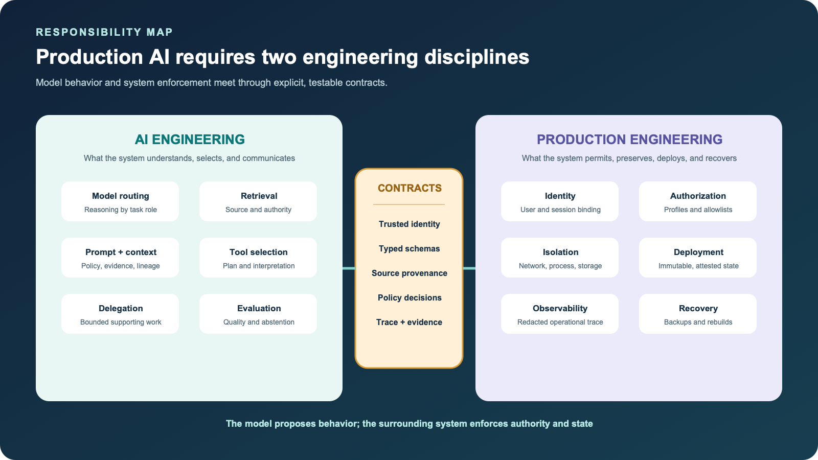
One of the most useful ways to reason about the system is to separate AI behavior from the software controls that make that behavior safe and operable.

AI engineering owns model routing, retrieval quality, prompt and context assembly, tool selection, delegated reasoning, abstention behavior, and nondeterministic evaluation. Production engineering owns identity, authorization, network boundaries, state durability, deployment, monitoring, backups, and recovery.

The two sides meet at explicit contracts. Retrieved content must include provenance. Tool calls must use typed schemas. Model routes must be declared and observable. Execution requests must carry a trusted identity and remain inside their assigned capability boundary. Evaluation failures must map back to an owning layer.

A responsibility map for a production AI assistant. AI engineering owns models, retrieval, prompts, context, tool selection, and evaluation. Production engineering owns identity, authorization, isolation, deployment, observability, and recovery. Typed and observable contracts connect the two sides. — The model can propose a plan, but software controls decide which identity, data, tools, and execution paths are available. Production reliability depends on both disciplines.

A request through the system

Consider an employee asking why an automated process did not complete.

First, the chat gateway binds the message to the authenticated employee and thread. The profile router selects a support profile whose default access is read-only. The controller retrieves relevant personal context and searches the shared knowledge base for the documented workflow.

If documentation answers the question, the assistant can respond with the source. If the employee is asking for a causal diagnosis, the controller uses diagnostic tools to inspect the available evidence. It traces the submitted input, effective configuration, owning code path, and chronological result. A queued record does not count as an execution attempt, and a configuration value does not prove that a running component consumed it.

If repository inspection is required, the support profile can search an approved read-only mirror. If a bounded command is necessary and authorized, the controller dispatches it to the isolated runner. The runner returns output without gaining access to the controller’s memory or secrets.

The controller then constructs the response from the evidence returned by those tools. If a decisive stage cannot be observed, the answer identifies the gap and the next useful check. If the request requires a privileged change, the system produces a handoff instead of silently widening its own authority.

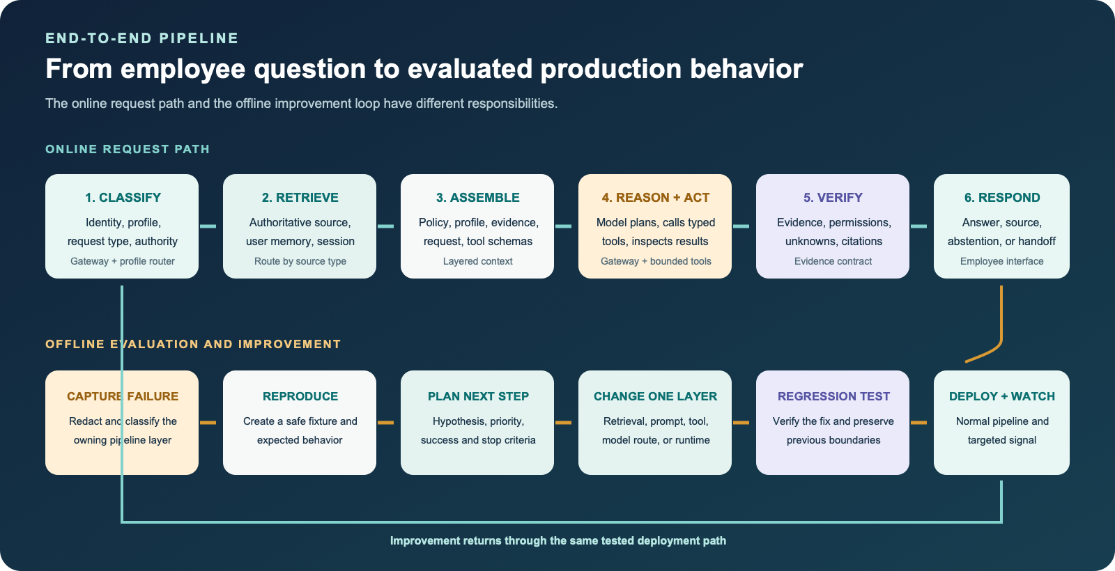
An end-to-end production AI pipeline. The system classifies the request, retrieves from authoritative sources, assembles context, routes to a model, executes typed tools when needed, verifies evidence and policy, returns a response, and feeds redacted failures into evaluation and improvement. — The online request path runs from classification through retrieval, reasoning, tool execution, and verification. The offline path converts observed failures into evaluations and regression tests.

Why I did not make every domain another agent

A common response to a large tool surface is to create a coordinator and a separate agent for every domain. That pattern can reduce tool confusion, but it also introduces additional prompts, model calls, shared-state questions, failure paths, and authorization surfaces.

I used profiles for trust boundaries and delegation for bounded work. The primary agent retains the task-wide plan, evidence, user interaction, and final response. A delegated model receives a small task only when its result can be checked independently. Tools remain grouped behind typed adapters and profile allowlists, so the primary agent does not need unrestricted access simply because the platform supports many capabilities.

This choice keeps coordination proportional to the problem. A new agent is justified when it needs a distinct objective, context, capability boundary, or independent lifecycle. A new tool category alone is not enough.

Where MCP fits

Model Context Protocol is one integration boundary in the system. It is useful when a capability should expose discoverable, typed operations through a service that owns authentication, validation, error handling, and API-specific behavior.

I do not treat MCP as a replacement for the rest of the architecture. Some capabilities are better implemented as local typed adapters. Command execution belongs in the isolated runner. Retrieval from the synchronized vault is a file and authority problem. Identity and authorization remain runtime controls. MCP helps standardize selected integrations, but it does not decide which user may call them or whether their results are trustworthy.

1. Retrieval choice: route by source and authority

I did not treat retrieval as a single vector-search problem. The system contains several knowledge types, and each one has a different owner, freshness model, and privacy boundary.

For shared policies and runbooks, I chose a synchronized Obsidian vault as the canonical source. Obsidian Headless keeps the runtime copy synchronized, while file and text search retrieve the relevant section directly. This preserves document structure and makes corrections visible to people. It also avoids presenting an embedding match as if it were an official policy.

For personal continuity, I used Honcho semantic retrieval backed by PostgreSQL and native pgvector indexes. The user identity comes from the authenticated Slack runtime, not from a name supplied in the prompt. Retrieval is filtered to that user before the result reaches the model.

For long conversations, I used Lossless Context Management as a separate context engine. It stores raw messages, builds hierarchical summaries, and retains source lineage. When older context becomes relevant, the agent can search the compacted history and expand the supporting messages. This is different from personal memory because it answers, “What happened earlier in this session?” rather than, “What should persist about this employee?”

For source code and technical documentation, lexical repository search is often more precise than semantic retrieval. Function names, configuration keys, error strings, and identifiers are exact evidence. The support profile searches an approved read-only mirror, while the engineering path can use its isolated workspace.

Web search and extraction are fallback sources for external information. Private SearXNG and Crawl4AI services return search and extracted content through controlled interfaces, while Camofox supports tasks that require browser interaction. Retrieved web content is treated as untrusted evidence, never as a new instruction.

The retrieval sequence is therefore authority-first. The router identifies the question type, searches the most authoritative eligible source, retrieves only the needed material, and records the source used. Semantic similarity helps find context, but it does not determine which source is allowed to define the answer.

2. Model selection rationale: spend reasoning where it matters

I separated model roles because the most capable model was not necessary for every operation.

The primary employee-facing Hermes agent uses a strong OpenAI reasoning model. I prioritized reliable tool calling, long-context behavior, code understanding, and the ability to distinguish evidence from inference. This model owns the task-wide plan, decides when tools are needed, evaluates their results, and writes the final response.

Delegated subtasks use a smaller model when the work is narrow and independently verifiable. Examples include extracting a constrained fact, comparing two bounded artifacts, or classifying a command for an approval workflow. The parent model retains the overall context and checks the returned result.

Memory derivation uses fast Google Gemini routes through a restricted gateway, while routine Hermes auxiliary tasks use smaller OpenAI models. These jobs run frequently, have structured outputs, and can be validated before their results enter future context. Embeddings use a dedicated OpenAI embedding model with a fixed dimension that matches the pgvector index.

This tiered approach reserves expensive reasoning for decisions that affect the employee while using smaller models for repeatable supporting work. It also makes cost and latency tunable without weakening every part of the system at once.

3. Brand and provider decision: managed, multi-provider, gateway-routed

I chose managed model providers rather than self-hosting the language models. The workload was conversational and uneven, and the system needed strong tool use and reasoning more than predictable continuous GPU utilization. Self-hosting would have added model serving, capacity planning, upgrades, and quality evaluation to an already complex production system.

The primary reasoning, delegation, and routine auxiliary routes use OpenAI models because tool calling, code-oriented reasoning, and Hermes integration were the strongest fit for the main workload. The Honcho memory subsystem uses Google Gemini models for frequent derivation and summarization work because those operations benefit from fast, economical inference. A managed OpenAI embedding model supplies vectors for semantic memory retrieval.

I did not scatter provider decisions through application code. Hermes configuration declares the main, delegated, and auxiliary routes. Honcho uses a separate, restricted AI gateway for memory derivation, summarization, and embeddings, with no tool access or fallback path. Credentials and route selection remain outside the employee conversation.

This design contains provider-specific behavior in one layer, supports fail-closed routing, and makes a later model evaluation possible without rewriting the chat, tool, or memory services. I still pin production routes rather than allowing an automatic provider fallback, because an unreviewed fallback can change latency, tool behavior, data handling, and output quality.

Cost is part of this routing decision. I would attribute usage by profile, model role, tool path, and request class rather than looking only at one provider invoice. That makes it possible to ask whether expensive reasoning improved a measurable failure mode, whether repeated retrieval created unnecessary context, or whether a delegated task cost more than handling it in the parent. A cheaper model is an improvement only when it preserves the required behavior.

4. Prompt design justification: separate authority from context

I used a layered prompt rather than one long set of instructions.

The first layer is the stable system policy, versioned in declarative profile files. It defines data handling, the difference between observation and inference, dangerous-action boundaries, and the requirement to acknowledge missing evidence.

The second layer is the profile contract. The support profile emphasizes plain-language answers, approved sources, read-only investigation, and escalation. The engineering profile includes a broader technical vocabulary and access to an isolated execution path. Each profile sees only the tools it is allowed to invoke.

The third layer is retrieved context. Personal memory, shared documentation, repository excerpts, and tool results are clearly marked as evidence. They do not gain authority to modify the system prompt or expand tool access. This matters because documentation, web pages, issue text, and source comments can contain instructions that were written for a person or can be actively malicious.

The fourth layer is the current request and typed tool schemas. Tool names, parameters, and return types tell the model what operations actually exist. Deterministic runtime checks then enforce canonical paths, authenticated identity, profile allowlists, confirmation state, and runner isolation outside the prompt.

For diagnostic work, I added an evidence contract to the prompt and tool output. A causal claim must identify the observed predicate, the code or workflow stage that consumes it, a counterexample or control when available, and whether the evidence is direct or inferred. When those fields cannot be supported, the model must keep the explanation as a hypothesis.

The prompt therefore guides reasoning and communication, while code and infrastructure enforce authority. That division lets the prompt remain useful without pretending it is a security boundary.

5. Evaluation and improvement: turn failures into regressions

I evaluated the assistant as a pipeline, not only as a model response.

The retrieval evaluation checks whether the system selected the correct source class, preserved user isolation, returned the relevant passage, and avoided using a less authoritative source when an approved source existed.

The reasoning evaluation uses representative questions with expected evidence and acceptable abstentions. It checks whether the answer distinguishes known facts from hypotheses, cites the inspected source, and asks for the next discriminating check when evidence is missing.

The tool evaluation checks correct tool selection, schema-valid arguments, read-only enforcement, path containment, timeout behavior, and safe handling of malformed tool output. Separate cases verify that a support request cannot reach engineering-only execution or another employee’s memory.

The context evaluation tests long sessions, repeated compaction, retrieval from summary lineage, and large tool results. The goal is to verify that the system can recover the supporting source after context has been compressed rather than trusting a summary with no drill-down path.

The deployment evaluation checks image immutability, profile rendering, policy configuration, infrastructure plans, service health, and runtime acknowledgement. A smoke test confirms that the deployed model route and tool surface match the approved configuration.

Layer	Example failure	Evaluation evidence
Retrieval	A less authoritative source overrides an approved procedure	Authority-ranked fixtures and expected passages
Identity	One employee retrieves another employee’s memory	Two-user isolation cases with distinct canaries
Tools	A support request reaches an engineering-only capability	Allowlist, path-containment, and denial tests
Reasoning	A hypothesis is presented as an observed fact	Evidence-contract cases with acceptable abstentions
Context	Compaction loses the source behind an earlier conclusion	Summary-lineage and source-expansion tests
Deployment	The infrastructure update succeeds but the old image keeps serving	Runtime generation and image-digest acknowledgement

I organize improvement as a closed loop: capture a redacted failure, classify the owning layer, reproduce it with a safe fixture, change the smallest responsible component, add a regression test, deploy through the normal pipeline, and watch the relevant operational signal. This prevents a retrieval problem from being “fixed” with a prompt change or an authorization problem from being hidden by a model retry.

The public version of this case study does not include performance or adoption numbers. The evaluation design is the defensible evidence I can discuss: what the system was tested to do, where it was expected to refuse, and how a failure became a durable improvement.

6. Next-step planning: make evaluation produce engineering work

An evaluation result is useful only if it changes what the team builds next. I treat next-step planning as the final stage of the pipeline rather than an informal note after testing.

The primary agent retains task-wide planning and final ownership. Delegated models receive only small, clearly scoped tasks whose outputs can be checked independently. This keeps the overall objective, evidence, and tradeoffs in one place instead of allowing several agents to make incompatible architectural decisions.

For each observed weakness, I create a bounded next step with six fields:

Observed failure: What happened, and at which pipeline layer?
Evidence: Which redacted trace, fixture, source, or runtime signal demonstrates it?
Hypothesis: What is the smallest plausible cause that can be tested?
Proposed change: Which single component should change first?
Success and stop criteria: What result would support the change, and what result would cause me to stop or change direction?
Regression coverage: Which existing privacy, authorization, retrieval, or deployment behavior must remain intact?

I then prioritize the work by user impact, security risk, recurrence, evidence quality, and implementation cost. A privacy-boundary or authorization failure outranks a stylistic answer problem. A repeatable retrieval failure outranks an anecdotal preference. A proposed model upgrade competes against prompt, retrieval, and tool fixes rather than becoming the default response to every weakness.

The resulting loop is: observe, classify, plan, implement, verify, deploy, and watch. This planning step is what turns an agent demonstration into an engineering system that can improve without losing the boundaries already established.

What one production request must reveal

Infrastructure health cannot explain why an answer was wrong. A production trace needs enough redacted information to reconstruct the decision path without turning the logging system into another sensitive-data store.

For each request, I want to identify the request and session, authenticated profile, retrieved source identifiers, model route, delegated tasks, selected tools, validated argument shapes, policy decisions, execution status, response classification, latency, and attributable model usage. Payloads that contain secrets, private conversation content, or sensitive operational data should be omitted or redacted before they reach monitoring.

This trace connects evaluation to operations. If a response used the wrong source, I can investigate routing and retrieval. If the correct tool was denied, I can inspect the profile policy. If the expected image was not serving, I can inspect deployment reconciliation. Observability becomes evidence about the pipeline rather than a large collection of unrelated logs.

The hardest choice: one interface, multiple trust boundaries

The most difficult design choice was whether to build one highly capable assistant or several narrow assistants. A single assistant is easier for employees to discover, but a universal toolset creates unnecessary authority. Separate applications make permissions clearer, but employees have to decide which system understands their question before they can ask it.

I chose one conversational experience backed by multiple profiles. The profiles share the gateway and selected knowledge services, but they do not share the same tools or execution path.

The support profile emphasizes explanation, retrieval, and evidence. It can read approved documentation and repository mirrors. General code execution and broad write access are absent. When support needs to perform a narrow write, such as proposing a shared-document update, it uses a purpose-built operation with a preview, fresh confirmation, one-time proposal, and audit record.

The engineering profile can use a broader toolset and a dedicated sandbox. That access remains separate from the controller’s state and credentials. The sandbox can be replaced without losing conversations or memory.

This design added operational complexity because profiles, policies, and tests had to stay synchronized. It was still the better tradeoff. Capability boundaries became inspectable and testable, while employees kept a consistent entry point.

An annotated engineering decision: one entry point, separate authority

This is a public reconstruction of the design decision described above. It is not an internal decision record, production trace, or measured test result. The cases below show what I would require a reviewer to check without revealing an employer’s configuration.

Context: Employees should not need to select an application before asking a question, but a support question should not inherit engineering privileges.
Decision: Keep one authenticated chat entry point. Route into a support or engineering profile with its own tool allowlist. Keep command execution on an isolated runner rather than in the stateful controller.
Boundary check A: A support request to inspect an approved document or read-only repository can use the corresponding bounded retrieval tool. A request to run a general command through the support profile must be denied or handed off, even if the prompt claims urgency.
Boundary check B: A user’s request for personal context must use the identity supplied by the authenticated gateway. A name or identifier written inside the message must not switch the memory identity to a different employee.
Boundary check C: An engineering-profile execution request must be validated before dispatch. The isolated runner should receive only the bounded task and permitted mounts, not the controller’s session database or credentials.
Tradeoff: Profile-specific permissions and isolation require more configuration and regression coverage than one universal assistant. They make the authority boundary reviewable without splitting the employee-facing experience.

These are design acceptance checks, not a claim that the public post exposes a passing test suite. The missing public evidence remains employer-specific traces, configuration, adoption data, and measured evaluation results.

How I handled failures

“The assistant failed” is not a useful operational category. I separated failures by the layer that owns the recovery.

A reasoning failure occurs when the evidence does not support a conclusion. The response remains explicit about unknowns and can request a discriminating check.

A policy denial occurs when a profile is not permitted to use a tool or path. The system returns a handoff or a narrower alternative. It does not treat a correct denial as an infrastructure outage.

A tool failure includes a connector timeout, malformed response, unavailable source, or validation error. The controller records the tool and stage that failed, while keeping sensitive payloads out of logs.

An execution failure occurs inside the isolated runner. Because the runner is disposable, the system can terminate the container, preserve bounded output, and retry only when the operation is safe to repeat.

A deployment failure occurs when infrastructure changes but the expected runtime does not converge. The deployment pipeline uses immutable images, a serialized reconciliation lease, and a runtime acknowledgement containing the expected generation and image digest. A successful infrastructure command is not enough to declare the deployment healthy.

A state failure affects conversation data, personal memory, shared knowledge, or a derived index. The recovery plan identifies which store is authoritative. Transaction-consistent backups protect primary state, and rebuildable indexes are regenerated after restore.

These distinctions also shaped monitoring. Dashboards and alerts cover service health, controller errors, and redacted incident events. They do not claim to measure answer quality. Diagnostic correctness is checked through evidence contracts and evaluation, not inferred from CPU utilization or an HTTP health check.

What I learned

The first lesson was that an AI assistant is an identity and permissions system before it is a conversational product. The answer is only trustworthy if the system can explain whose context it used, which source it treated as authoritative, and which capabilities were available.

The second lesson was that memory needs separate ownership domains. Personal continuity, shared organizational knowledge, active conversation context, and long-session retrieval solve different problems. Combining them into one store makes privacy, provenance, and correction harder.

The third lesson was that tool use needs stronger contracts than natural-language guidance. Typed inputs, path containment, read-only mounts, purpose-built writes, isolated execution, and independent policy checks make the boundary enforceable.

The fourth lesson was that production deployment needs evidence. Infrastructure as code describes the intended state. Runtime attestation shows what is actually serving requests. Both matter for a stateful assistant whose model, tools, and permissions can change independently.

The final lesson was about product design. Employees do not need to see every internal component, but the system should make its uncertainty and limits visible. A concise answer with a source, a bounded investigation, and an honest handoff are all successful outcomes when they match the evidence and authority available.

This project brought together the parts of engineering I enjoy most: backend architecture, AI integration, security boundaries, infrastructure, observability, and the careful translation of a complex system into a simple employee experience.

Making the Twin Forge Observable

October 9, 2026

How I connected a Hermes research workflow to Discord so I can follow its decisions and inspect the evidence behind them.

In my previous post, I introduced the Twin Forge, a small research team I built with Hermes to investigate uncertainty in cancer digital twins. The scientific goal is still demanding: establish a credible forecasting model, then test whether a sequential uncertainty layer can make its predictions more useful. Building agents that propose and run experiments was only part of the problem. I also needed to know what the workflow was doing while I was away from the terminal.

Giving each role a job

The first version had a Scientist and an Engineer. The Scientist chose the next experiment and interpreted the result. The Engineer implemented and ran it. That loop exposed a weakness: code completing successfully did not tell me whether the experiment followed its specification or whether the conclusion was justified.

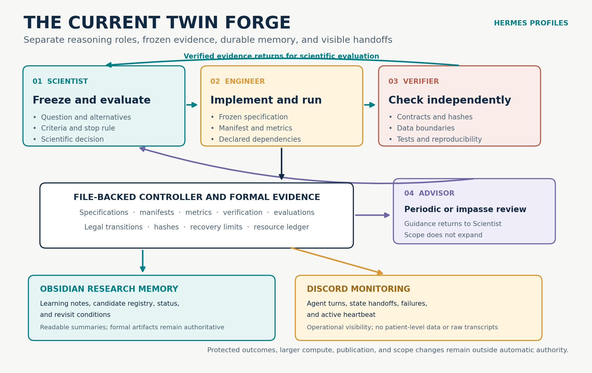
I added a Verifier to check the implementation, artifacts, and data boundaries independently before the Scientist evaluates the result. An Advisor now checks in periodically and helps when the Scientist reaches an impasse. The Scientist still leads ordinary planning. The Advisor is there for guidance, not to prescribe every experiment.

The resulting loop has a deliberate order: the Scientist freezes a question and success criteria, the Engineer runs that experiment, the Verifier checks the evidence, and the Scientist decides what the verified result means. If the Scientist is stuck, the Advisor can help identify a different route. Each role has a purpose, and each handoff leaves a record.

The monitoring problem

An automated research loop can look active while making little progress. A long compute job might be running normally, an agent might be retrying an operational error, or the workflow might have stopped at a decision point. Those situations need different responses, but they are easy to confuse if the only view is a terminal transcript or a file that I have to remember to open.

We ran into concrete versions of that ambiguity. Questions about the provenance of pretrained weights stopped one proposed use of the segmentation model. A separate compatibility failure occurred before a model forward pass, so there was no scientific result to interpret. Other experiments reached an authorized cycle limit or a frozen scientific stop rule. From a distance, each case could look like “the agents stopped.” In reality, one called for evidence about the weights, another for a technical repair, and another for a research decision. I needed the workflow to tell me which situation I was looking at.

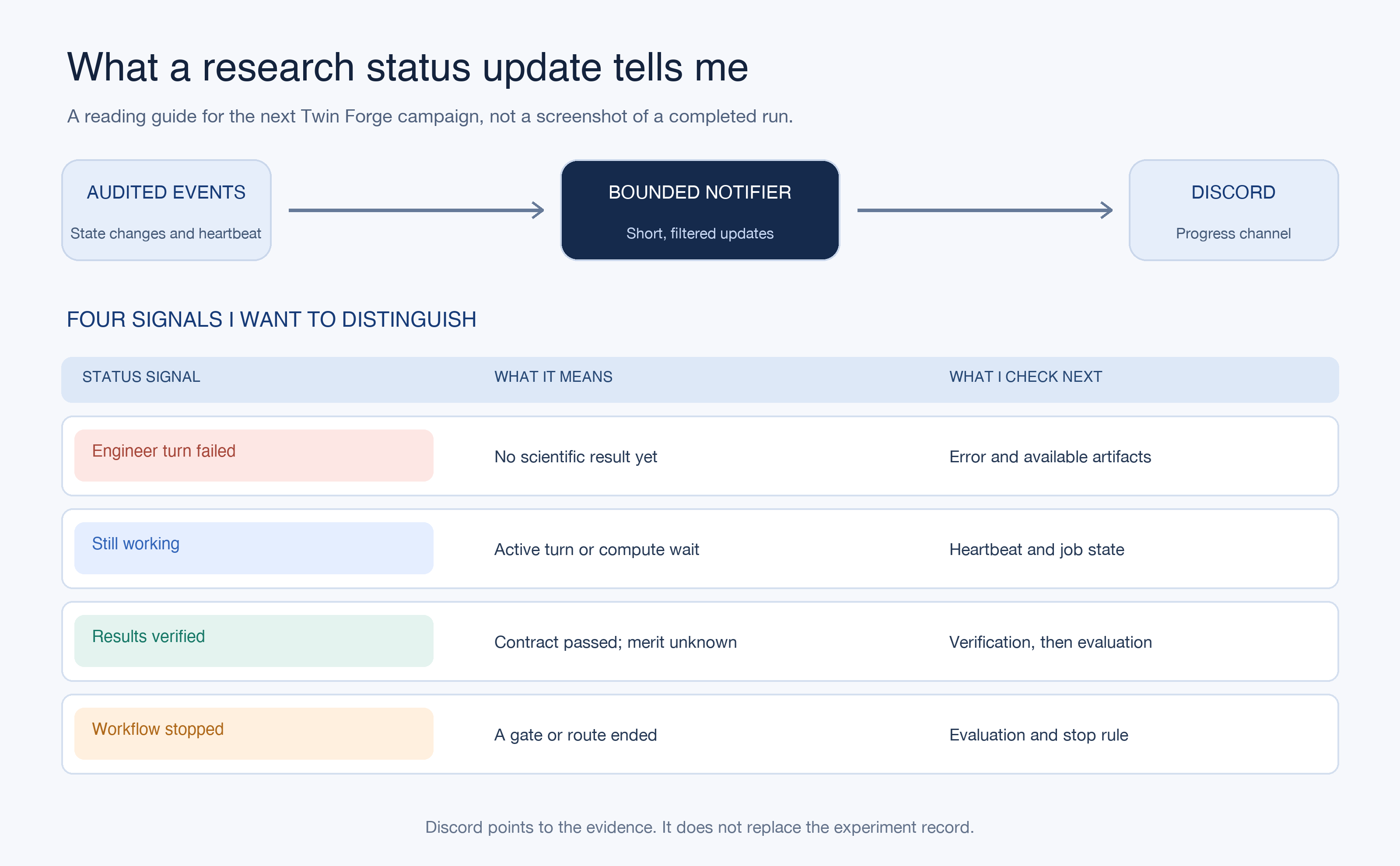
There is also a scientific distinction that a simple “done” message misses. An Engineer finishing a run means that outputs exist. A Verifier passing means that the run satisfies the frozen contract. A Scientist evaluating the result means that the evidence has been compared with the scientific criteria. A negative result can be valid and informative. A failed verification is an implementation or evidence problem. I want the monitoring system to preserve those differences.

Connecting Hermes to Discord

I connected the workflow to a dedicated Discord research channel. Hermes still runs the research roles, while a small notifier reads the workflow controller's recorded events and heartbeat. It reports when the Scientist, Engineer, Verifier, or Advisor starts and finishes a turn, when a turn fails, and when the workflow changes state or research route. During a long agent turn or compute wait, it also sends a periodic “still working” update. The diagram below is a guide to interpreting those updates in the next campaign.

This is a guide to future status messages, not a screenshot of a completed run. Each message points back to the experiment record.

This design keeps Discord as a window into the workflow rather than the source of truth. Experiment specifications, run manifests, metrics, verification reports, and evaluations remain in the research repository. Obsidian presents the learning record in a form I can read across experiments. The Discord channel gives me timely signals and experiment identifiers so I know which evidence to inspect. I can also ask the separate research bot for a current status summary drawn from those records.

The notifications are intentionally short. They do not copy full agent conversations, raw logs, credentials, or patient-level information into Discord. A notification outage also does not change the scientific state or stop an experiment; the notifier can retry from its last recorded position.

What I hope to learn from the stream

The most useful status update may be a handoff. It tells me who owns the next step and whether the workflow is moving through planning, execution, verification, and evaluation as intended. A sequence of repeated failures may reveal a dependency or compute problem. A verified negative result may tell me to stop tuning one model and test a different hypothesis. In either case, the short Discord message points back to the detailed record rather than pretending to be the analysis itself.

My aim is a more effective agentic flow, not merely a busier one. Clear status makes it possible to repair an operational problem without quietly changing the experiment, to ask the Advisor for a new direction when the Scientist is stuck, and to honor a scientific stop rule when the evidence does not support another run. It also makes my own interventions more focused. I can ask why an experiment stopped, what was independently verified, and what evidence would justify the next route.

The Discord connection and setup message have been tested. The automatic per-agent stream is wired to the next workflow run, so I have not yet treated it as evidence that a full campaign has been monitored end to end. That is the next operational check. The larger research question remains open, but the process for asking it is becoming easier to observe, audit, and improve.
Agentic AI Researcher

October 7, 2026
How the Twin Forge evolved from a two-agent experiment into an evidence-driven research workflow.

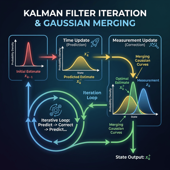
My goal is to develop a proof of concept for uncertainty quantification in cancer digital twins. The proposed uncertainty layer combines particle filtering with a Kalman-family conditional update. Particles can represent nonlinear, multimodal, or discrete uncertainty, while a conditional update can handle suitable continuous states. Before any of that is useful, I need a forecast model that deserves to have uncertainty placed around it.

That requirement has shaped the research more than any particular algorithm.

My industry work in production AI and backend engineering influenced how I approached the problem. A promising model is only one part of a dependable system. Inputs, state, failure modes, tests, recovery, and monitoring all have to be explicit. Research requires the same discipline, with an additional distinction: code that runs is not necessarily evidence that supports a scientific claim.

I first explored a breast-cancer digital twin based on a reaction-diffusion partial differential equation, or PDE. The mathematical framework was promising, but the data available to me did not contain all of the patient-specific inputs and longitudinal measurements needed to reproduce the model as intended. I then moved to brain metastases, where I had longitudinal imaging work, lesion annotations, and a pretrained segmentation model from a separate NYUMets reproduction project.

The move did not make the problem simple. A patient may have several lesions. Existing lesions can grow, shrink, disappear from an image, or become difficult to match across irregular visits. New lesions may become visible between scans, but the first visible date is not necessarily the biological start time. Treatment may also occur between observations. A segmentation network can help define what is visible at a visit, but it does not automatically predict the next visit.

I needed a research process that could examine these possibilities without confusing a plausible mechanism with a validated forecast. That is why I built the Twin Forge.

Version one: the Scientist and the Engineer

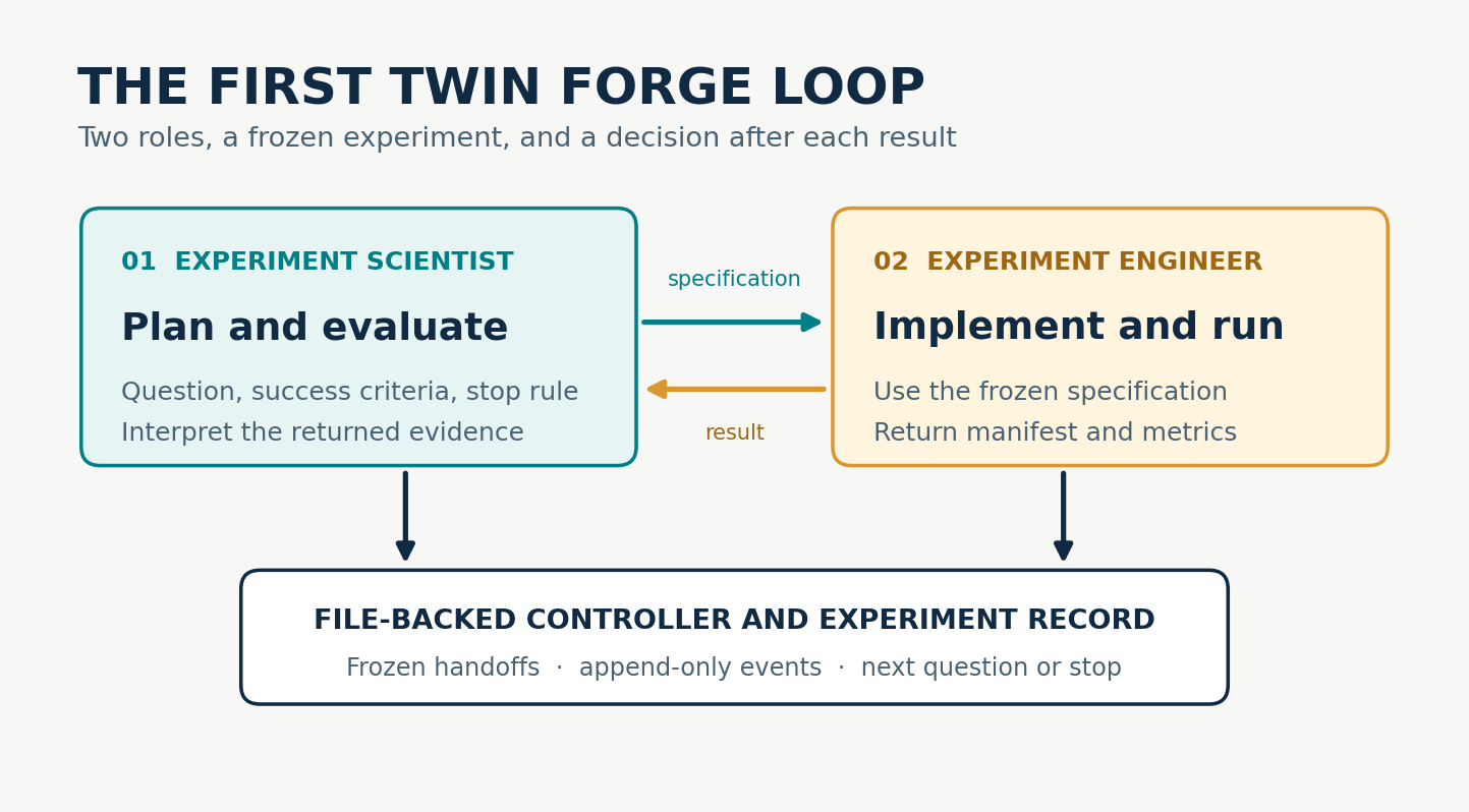
The first workflow used two Hermes profiles: an Experiment Scientist and an Experiment Engineer.

The Scientist selected a bounded question, stated the success criteria, and decided what the result meant. The Engineer implemented the experiment, ran it, and returned the code, manifest, and metrics. The result then went back to the Scientist for another round of planning.

This gave the work more structure than a single open-ended agent conversation. The roles had different responsibilities, and the experiment specification created a record of what was supposed to run. A file-backed controller tracked the handoff so that completed evidence could not be silently rewritten as a different experiment.

The first loop was simple:

Scientist plans → Engineer runs → Scientist evaluates → next experiment or stop

The idea was to let the Scientist explore several routes, including a constrained PDE, a reduced-state transition, a compact temporal model, and synthetic known-truth tests for the future uncertainty layer. Hermes provided the role-specific agents and tools, while the repository held the actual research record.

The first Twin Forge separated scientific planning from implementation, with the experiment record connecting the two roles.

What the first loop exposed

The two-agent workflow ran into problems that looked similar from the outside but had very different meanings.

A missing dependency or incompatible environment was an execution failure. Unclear provenance for pretrained weights was an evidence problem. A request to retrain a backbone or open protected outcomes was a scope decision. A model failing to outperform persistence was a scientific result. In the early workflow, each could appear as the same message: the agents stopped.

The loop also lacked an independent check between implementation and interpretation. A command completing successfully did not prove that the Engineer used the frozen data boundary, preserved the forecast origin, produced the required artifacts, or evaluated the correct endpoint. The Scientist could read the result, but the same role that wanted to advance the research was also deciding whether the handoff was trustworthy.

Another problem was memory. A long transcript could explain what happened during one turn, but it was not a durable scientific record. Without a structured account of supported findings, limitations, stopped candidates, and revisit conditions, the workflow could keep proposing small variations of an idea that had already failed.

Finally, the workflow was difficult to observe. A long-running job, an agent retry, a failed verification, and a completed negative result require different responses. I needed to know which state the research was in without continuously watching a terminal.

These were architecture problems, not prompting problems. Adding a longer instruction to the same two roles would not create independent verification, durable evidence, or operational visibility. This is where my experience with production systems became especially relevant. Reliable workflows separate responsibilities, make state visible, constrain retries, and preserve enough evidence to explain a failure after it occurs.

Version two: separating evidence from interpretation

The next version added an Experiment Verifier and made the experiment contract stricter.

The Scientist now freezes the research question, data boundary, alternatives, success criteria, and stopping rule before implementation. The Engineer runs that specification and writes a manifest and aggregate metrics. The Verifier independently checks the frozen contract, artifact hashes, tests, data boundaries, and reproducibility. Only after verification passes does the Scientist evaluate the scientific result.

Each role has a boundary:
- The Engineer cannot verify its own output.
- The Verifier cannot repair the code or decide that the research should advance.
- The Scientist cannot reinterpret an unverified run as scientific evidence.
If verification fails, the original artifacts remain unchanged. An eligible repair receives a new experiment identifier and uses a bounded recovery path. A negative scientific result can close one candidate while allowing the Scientist to test a materially different candidate. This prevents operational recovery from quietly changing the hypothesis, endpoint, or success criteria.

The file-backed controller enforces the legal state transitions. It freezes specification digests, assigns the next owner, records append-only events, tracks resource use, and stops when the campaign reaches a scientific or operational boundary. Hermes provides the role-specific reasoning and tools, but the controller and experiment artifacts determine what happened. This separation is similar to a production control plane: the agents perform the work, while an external state machine governs what transitions are allowed and records why they occurred.

Adding an Advisor without taking planning away from the Scientist

I wanted the Scientist to lead ordinary planning, much like a PhD student develops and tests ideas between advisor meetings. I did not want every experiment prescribed by a supervisory agent.

The Research Advisor therefore enters at specific points. It checks in after every third completed cycle and reviews the workflow when the Scientist reaches an impasse. The Advisor reads the original research objective and the current aggregate evidence, then recommends whether the Scientist should pursue another authorized route or stop. An advisor memo is guidance, not a new experiment specification and not permission to expand the scope.

This relationship gives the Scientist room to work while still creating a path out of repetitive or unproductive planning. It also distinguishes a research impasse from a technical failure that the Engineer should repair.

The agents exchange specifications and evidence through the repository. Obsidian and Discord make the work easier to understand, but neither replaces the formal experiment record.

Obsidian as research memory

Hermes conversations are useful for reasoning, but they are not the source of truth. Every formal experiment has a specification, run manifest, metrics, verification report, and scientific evaluation. The controller records the state transitions and preserves the hashes of active artifacts.

I use Obsidian as the readable layer over that evidence. After a completed evaluation, the workflow creates or refreshes a learning note that records what the experiment supports, what it does not support, which assets are reusable, and what evidence would justify revisiting the idea. A candidate registry prevents the Scientist from repeating a stopped approach merely by changing a threshold, seed, or parameter.

This design lets memory compound without turning an old note into a new fact. When an Obsidian summary and a formal experiment artifact differ, the formal artifact remains authoritative.

Discord as the monitoring surface

The next improvement was visibility. I connected the workflow to a dedicated Discord research channel. A notifier reads the controller’s append-only events and active heartbeat, then reports when each role starts or completes a turn, when a handoff changes state, when a failure occurs, and when a long-running step is still active.

Discord is a window into the workflow, not the workflow itself. It does not receive patient-level data, protected images, credentials, or full agent transcripts. A notification failure does not alter the experiment state. The messages provide enough context to distinguish an active job, an execution failure, a verification failure, an advisor review, and a scientifically valid stop.

I also created separate Discord-facing bots for research status and workflow coordination. They read the repository’s current state and aggregate records rather than inventing progress from conversation history.

Why the new architecture is an improvement

The current design improves the research process in five ways.

First, it makes claims traceable. A conclusion points back to a frozen question, implementation record, verification report, and evaluation.

Second, it separates kinds of failure. The workflow can respond differently to an environment problem, an evidence problem, a failed scientific criterion, and an exhausted research route.

Third, it supports bounded autonomy. The agents can plan and run several experiments without requiring me to supervise every handoff, while campaign limits, data boundaries, resource budgets, and stopping rules remain explicit.

Fourth, it preserves negative results. A candidate that fails its frozen criteria is recorded as stopped, along with the evidence required to revisit it. The workflow cannot manufacture progress by repeatedly tuning the same failed idea.

Fifth, it makes the work observable. Obsidian explains what the research has learned across experiments, while Discord shows what the system is doing now.

What the workflow taught me about the science

The architecture did not solve the digital-twin problem by itself. It made the limits of the current evidence harder to ignore.

The experiments showed that persistence is a meaningful baseline and that a mechanistic model does not earn credibility merely by generating plausible trajectories. Synthetic experiments also separated predictive usefulness from parameter recovery. A model may produce a reasonable forecast while its growth and diffusion parameters remain poorly identified.

The most recent campaign tested whether released masks and existing metadata could support an operational MRI-visible burden forecast before attempting the particle and Kalman-family uncertainty layer. The workflow stopped because the required geometry and forecast prerequisites were not established within the authorized evidence. Without an adequate center forecast, the real-data uncertainty experiment was not admissible.

That is a useful research outcome. The system did not continue running increasingly complicated models simply because more cycles were available. It preserved the negative gates and identified what new evidence would be needed to reopen the route.

What comes next

The next step is not to place a sophisticated uncertainty method on top of an unsupported forecast. I need either stronger longitudinal evidence, a better-defined observation and geometry contract, or a different digital-twin foundation that can be evaluated against simple alternatives.

The Twin Forge is still a work in progress, but its purpose is now clearer. It is not an automated discovery claim. It is an evidence-driven research system that helps me plan, execute, verify, remember, and monitor a difficult scientific program.

That architecture gives me a better chance of producing a defensible proof of concept. It also gives me a principled way to conclude that a proposed route is not supported by the available data.

For a closer look at the monitoring layer, see Making the Twin Forge Observable.
Designing Event Driven Python Systems for Reliable AI Workflows

September 30, 2026
An API endpoint can make an AI workflow look simpler than it is. A request arrives, Python calls a model or another service, and a response comes back. That design works until the job also depends on document processing, image analysis, external APIs, database updates, or a downstream operational action. Then one request may outlive a web connection, cross several service boundaries, and partially succeed before anything reports an error.

The difficult question is no longer, “Can the model produce the right output?” It is, “Can the system determine what happened, resume safely, and avoid doing the same consequential work twice?”

I have built asynchronous Python services using queued workers and PostgreSQL state tracking, and I have maintained Apache Airflow workflows that coordinate data retrieval, classification, database updates, retries, and monitoring. Across those systems, the most reusable reliability patterns were not specific to the model. They were ordinary distributed systems practices applied carefully around probabilistic components.

This article describes those patterns at a general level. It intentionally omits proprietary architecture, customer information, internal endpoints, and performance claims.

An event driven design is useful when it makes incomplete work visible, recoverable, and safe to repeat.

Give every unit of work an identity

The first requirement is a durable job identifier. A browser connection, worker process, or queue delivery is temporary; the logical job is not. The identifier should be created when the application accepts the work and then travel through every event, log entry, state transition, and output record associated with that work.

A practical workflow also needs explicit states. The exact names vary. A request enters received after initial validation and assignment of a durable identifier. It becomes queued after the application records an event for asynchronous processing. It becomes running after a worker claims a particular attempt. It may enter waiting while progress depends on an external system or a scheduled continuation. It becomes completed after the expected output and final state are persisted. It enters retryable_failed when an attempt fails under conditions that may change. It enters manual_review when continuing automatically would be unsafe or ambiguous. It enters terminal_failed when another automatic attempt is not expected to succeed.

These states are not decorative labels. They define which transitions are allowed and which component is permitted to make each transition. If any worker can overwrite any state, the database becomes a log of competing opinions rather than a source of truth.

Persist intent before depending on delivery

A reliable API should not acknowledge work that exists only in memory. A common sequence begins by validating the request. The application then creates the durable job record and records the event that needs to be published. It publishes or dispatches the work only after that state exists. Finally, it returns the stable job identifier.

The database write and message publication are separate operations, which creates a problem with two related writes. The application can persist the job and fail before publishing, or publish the event and fail before recording the corresponding state. For work that cannot be silently lost, a transactional outbox is one useful pattern. The job and an outbox record are committed together, and a separate publisher delivers unsent events. This does not eliminate failure, but it turns an invisible gap into state the system can inspect and reconcile.

The queue should transport intent, not become the only record that the intent existed. Queues are designed to move work. The database should answer what the system currently believes about that work.

Treat the event as a versioned contract

An event should be more deliberate than an arbitrary Python dictionary. At minimum, consumers need enough information to identify the logical job, identify the individual event, interpret the schema, correlate activity across services, and locate the necessary data.
```
from datetime import datetime
from uuid import UUID

from pydantic import BaseModel, Field


class WorkEvent(BaseModel):
    event_id: UUID
    job_id: UUID
    event_type: str
    schema_version: int = 1
    attempt: int = Field(ge=0)
    occurred_at: datetime
    correlation_id: str
    payload_ref: str
```
The event can carry a reference to durable input instead of copying a large or sensitive payload through every transport. That keeps contracts smaller, reduces duplicated data, and makes access control easier to reason about. The tradeoff is that the referenced data must remain available and versioned long enough for retries and reprocessing.

Schema versions matter because producers and consumers rarely change at exactly the same time. A worker should reject or route an unsupported version explicitly rather than misinterpreting it as the current structure.

Design for duplicate delivery

Many message systems guarantee that a message will be delivered one or more times. That is useful, but it means a consumer may receive the same logical work more than once. Duplicate delivery is not an unusual edge case. It is part of the contract.

Idempotency means that repeating the same logical operation does not create a second, conflicting outcome. It usually requires more than checking whether an event identifier appeared before. The application must define what “the same logical operation” means at the business boundary.

Several controls work together. A unique idempotency key can identify the logical action. A receipt table can enforce a uniqueness constraint on processed events. Conditional state transitions can succeed only from an expected prior state. Database transactions can persist the result and completion state together. When an outside action supports it, the application can use an external provider key or look up an existing result before creating another one.

In a reusable OCR service, for example, I used idempotent database updates so that retrying processing did not create contradictory records. The same principle becomes more important when a workflow can send a message, create a case, or initiate another externally visible action.

An important distinction is that deduplication and idempotency are not identical. A deduplication cache may forget an old event. An idempotency rule at the business level should still protect the operation if that event returns later.

Retry only failures that may become successful

“Retry on exception” is not a recovery strategy. Some failures are transient: a connection reset, rate limit, temporary provider outage, or database lock may succeed later. Other failures are deterministic: a malformed event, unsupported schema, missing authorization, or invalid record reference will usually fail in the same way on every attempt.

The worker should classify failures and record a structured reason. Retryable failures can use bounded attempts, exponential backoff, and jitter. Deterministic failures should move to a terminal or review state quickly enough to avoid wasting capacity and hiding a problem with data quality behind repeated noise.

Model outcomes need their own classification. A valid response may still be inconclusive, fail a domain constraint, or require review. That is different from a network error and should not automatically enter the same retry loop. Retrying the identical model request may only produce a different answer without resolving the underlying ambiguity.

When a worker exhausts its retry policy, the event should not disappear. A dead letter route or durable failure state should preserve the job identifier, event type, attempt count, last structured error, and enough context for safe replay or manual review.

Make state transitions conditional

Two workers can observe the same job before either finishes updating it. A simple protection is to make state transitions conditional on the state the worker expected to find.
```
UPDATE jobs
SET status = 'running',
    attempt = attempt + 1,
    started_at = CURRENT_TIMESTAMP
WHERE id = :job_id
  AND status IN ('queued', 'retryable_failed');
```
If the update affects no rows, the worker does not own that transition. It should stop, inspect the current state when appropriate, and avoid performing the external action.

Tasks that run for a long time may also need a lease or heartbeat. Without one, running can mean either “healthy work is in progress” or “the worker disappeared yesterday.” A lease makes ownership temporary, while reconciliation can identify abandoned attempts and return eligible jobs to a recoverable state.

Use Airflow and event driven workers for different jobs

Event driven services and workflow orchestrators solve related but different problems.

Queued workers are a strong fit when work arrives irregularly through an API or external event, when individual jobs should begin quickly, and when services need to scale independently. The message boundary separates request intake from processing and lets each consumer handle a bounded unit of work.

Airflow is a strong fit for scheduled workflows or workflows with many dependencies. It can retrieve data, prepare inputs, run classification, persist results, generate reporting artifacts, and monitor whether the expected sequence completed. Its DAG makes dependencies, retries, schedules, and historical runs visible.

The two approaches can work together. An event driven service can persist operational work as it arrives, while Airflow handles periodic aggregation, reconciliation, backfills, or batch processing with several stages. The key is to avoid giving both systems ambiguous ownership of the same transition. Each boundary should have a clear source of truth and a clear recovery path.

Observability should follow the job

A request identifier that disappears at the queue boundary is not enough. The correlation identifier should connect the API request, published event, worker attempt, database transitions, dependency calls, and final outcome.

Useful operational signals include queue age, not only queue length. They include time spent in each workflow state, attempt counts, retry reasons, and jobs that remain running beyond their lease. They also include dead letter volume, manual review volume, schema version mismatches, model outputs rejected by deterministic validation, and dependency failures separated from application failures.

These measurements should be reported as actual observations, not assumed guarantees. I have worked primarily on reliable execution and operational visibility; I would not attach a p95 or p99 claim to a system unless that latency had actually been measured under a defined workload.

Logging also requires restraint. A trace should make behavior reconstructable without duplicating prompts, customer records, credentials, or sensitive payloads into a loosely governed logging system. Stable identifiers, state transitions, result classes, dependency timings, and carefully selected metadata are often more useful than a full content dump.

Test the failures the architecture claims to survive

Tests of successful execution prove that the components can cooperate once. Reliability tests should force the boundaries to misbehave.

I would include several failure cases. The same event may be delivered twice. A worker may stop after an external action but before acknowledging the message. A database update may succeed while event publication is interrupted. An old event may arrive after the job has already advanced. A consumer may receive an unsupported schema version. An external request may time out even though the provider completed it. A retry may begin while another worker still holds a valid lease. Reconciliation may also encounter a job whose state conflicts with its external outcome.

These scenarios reveal whether the system has real recovery behavior or only a retry button. They also clarify where an automated retry is safe, where a compensating action is possible, and where the correct response is to stop and request human review.

Reliability is the product of explicit boundaries

Event driven architecture does not make failure disappear. It makes failure observable and gives the application places to respond deliberately.

The API owns validation and durable acceptance. The event contract owns the handoff. The worker owns one bounded attempt. The database owns durable workflow state. The orchestrator owns declared dependencies. Reconciliation owns the gap between what should have happened and what the system can prove happened.

That separation is especially valuable in AI systems. The model can remain probabilistic while the surrounding application enforces deterministic rules about identity, authorization, state, retries, and consequential actions. The result is not a workflow that never fails. It is a workflow that can explain its state, recover safely, and keep incomplete work from becoming invisible.

Next in this series: visual similarity and OCR at scale.
What It Takes to Move an LLM Application from Demo to Production

September 29, 2026
An LLM demo can be convincing after only a few hours. It accepts a prompt, produces fluent language, and makes the underlying model look like the product. Production changes the question. The system now has to assemble the right context, preserve state, call tools safely, recover from partial failures, and produce useful behavior repeatedly—not only during a carefully chosen example.

At Gray Falkon, I built and maintained the Python backend for a customer-facing AI assistant that combined document retrieval, product context, conversation management, and tool-assisted reasoning. I also worked on LLM-powered messaging services for classification, translation, and response generation inside broader operational workflows. The applications differed, but the engineering lesson was consistent: the model call was only one component of the system.

This article describes the reusable engineering patterns at a general level and intentionally omits proprietary implementation details, customer data, and internal metrics.

The model generates language. The surrounding system determines whether that language is grounded, timely, recoverable, and useful.

Start with the operational job, not the model

The first design decision is not which model to use. It is defining the job the system must perform and the contract around that job. A production request usually contains more than a user message. It may also require account state, product records, retrieved documents, prior conversation turns, workflow status, authorization information, and rules governing which actions are allowed.

I treat the LLM as a probabilistic component inside a deterministic application boundary. The application owns input validation, data access, state transitions, permissions, persistence, and error handling. The model can interpret language, rank alternatives, or propose an action, but ordinary software should decide whether that action is valid and whether it may execute.

This boundary matters because product success is not the same as model fluency. A response can sound excellent while using stale context, selecting the wrong record, omitting a required action, or leaving the workflow in an inconsistent state.

Context assembly is a data-engineering problem

Retrieval-augmented generation is often summarized as “search, then place the results in the prompt.” That description hides most of the engineering work. The system must determine which sources are authoritative, which records belong to the current user or task, how fresh the information must be, how conflicting evidence should be handled, and what can fit within the available context budget.

A useful context pipeline produces structured evidence rather than an undifferentiated collection of text. For each retrieved item, the application should know its source, scope, version, timestamp when relevant, and relationship to the request. It should also be possible to distinguish “no relevant information exists” from “retrieval failed” and from “the system was not permitted to access that information.” Those states should not collapse into the same empty prompt.

The practical result is that retrieval deserves the same care as any other production data pipeline: validation, filtering, observability, regression tests, and explicit failure modes.

Conversation history is not application state

A transcript can help a model understand the immediate conversation, but it is a poor substitute for explicit state. Important facts should not exist only as sentences several turns back. The application should persist the identifiers, decisions, workflow stage, and durable outputs that later operations depend on.

This separation also makes the system easier to reason about. Conversation history answers, “What has been said?” Application state answers, “What is currently true, what has completed, and what may happen next?” The two can inform each other, but they have different consistency and retention requirements.

Database-backed state also supports recovery. If a worker stops, a provider times out, or a request is delivered more than once, the system can resume from a known transition rather than reconstructing reality from generated text.

Tool use needs a strict execution boundary

Tool calling makes an LLM application much more capable, but it also introduces risk. A generated function name or argument set is a proposal, not an instruction that should automatically be trusted. Before execution, deterministic code should validate the schema, confirm authorization, check relevant business rules, and reject incomplete or ambiguous arguments.
- Validate inputs: Types, required fields, permitted values, and referenced records must be checked outside the model.
- Make operations idempotent where possible: Retrying the same logical request should not create duplicate work or conflicting state.
- Bound execution: Timeouts, retry limits, and clear cancellation behavior prevent one dependency from holding the workflow indefinitely.
- Return structured results: The model should receive a compact success or failure object rather than guessing what happened from unstructured logs.
- Record consequential actions: Auditable transitions make debugging and review possible without treating the conversation itself as the system of record.
A useful rule is that the model may help decide what the user intends, while the application remains responsible for what the system actually does.

Asynchronous workflows change the architecture

Many AI workflows depend on slow or failure-prone services: document processing, browser-mediated operations, external APIs, database work, or downstream reporting. Keeping all of that inside a synchronous web request creates brittle latency and makes recovery difficult.

Event-driven Python services provide a cleaner boundary. The API can validate and persist a request, publish work for an appropriate consumer, and return a stable identifier. Workers can then perform bounded units of work and record their results. Orchestration can coordinate schedules and dependencies, while the database remains the durable source of truth.

This design does not eliminate failure; it makes failure representable. A workflow can be pending, running, complete, retryable, or terminally failed. That is far more useful than a long request that eventually disappears behind a generic timeout.

Assume partial failure

Production reliability comes from treating failure as an ordinary system state. The model provider may time out. Retrieved context may be missing. A queue may deliver an event more than once. A tool may succeed while its response is lost. A downstream service may reject a request after earlier steps have completed.

The response to each case should be designed before deployment. That may mean bounded retries with backoff, idempotency keys, transactional state changes, reconciliation jobs, explicit manual-review states, or a safe fallback that performs no action. The appropriate choice depends on the consequence of being wrong. Retrying a read is different from repeating an external action.

It is also important to preserve the difference between a model-level failure and a system-level failure. A structurally valid response can still be semantically poor, while a strong model response can be unusable because a dependency or state transition failed.

Evaluation has to cover the complete system

A single model benchmark cannot represent production quality. I prefer layered evaluation because each layer answers a different question:
1. Contract tests verify schemas, permissions, routing, persistence, and tool behavior.
2. Retrieval evaluations test whether the correct evidence is found and irrelevant evidence is excluded.
3. Behavioral test cases check expected responses across ordinary, ambiguous, and adversarial inputs.
4. Operational metrics measure latency, error rates, retry frequency, queue health, and dependency failures.
5. Human review examines qualities that remain difficult to reduce to one automatic score, including usefulness, tone, and whether the response is appropriately cautious.
Regression sets are especially valuable. Prompts, retrieval rules, tool schemas, application code, and model versions can all change behavior. A release should be tested against representative cases, including previous failures, rather than evaluated only through fresh demonstrations.

Observability must follow the request across boundaries

Traditional service monitoring remains necessary, but AI applications also need traces that explain how a result was assembled. Useful diagnostic context can include the request identifier, selected data sources, retrieval outcome, model and configuration version, tool calls, state transitions, timing, and a structured failure reason.

That does not mean indiscriminately logging prompts or sensitive content. Observability should be designed with data minimization and access control in mind. The goal is to reconstruct system behavior without creating a second, poorly governed copy of the underlying data.

The most valuable dashboards connect infrastructure symptoms to product behavior. A healthy process count is not enough if retrieval is returning empty context, structured outputs are failing validation, or a downstream tool is quietly rejecting requests.

What changed between the demo and the product

The demo centered on generation. The product required a much larger set of guarantees:
- The correct user, record, and workflow context had to be selected.
- Durable state had to live outside the conversation.
- Generated tool requests had to pass deterministic validation.
- Slow work had to move across asynchronous boundaries safely.
- Retries had to avoid duplicating consequential actions.
- Failures had to be visible, classifiable, and recoverable.
- Changes had to be tested across the full pipeline, not only at the model layer.
This is the part of AI engineering I find most interesting: connecting probabilistic model behavior to deterministic operational expectations. A useful production AI system is not merely a model wrapped in an API. It is a carefully bounded software system that knows where uncertainty belongs, where validation is mandatory, and how to remain understandable when something goes wrong.

Next in this series: Designing event-driven Python systems for AI workflows.
Particle Filters

June 4, 2026
Illustration of the particle filtering algorithm showing prediction, update, and resampling steps.

A particle filter is a method for estimating the hidden state of a system as that system changes over time.

That sounds similar to a Kalman filter, and it is. Both methods are used for filtering. Both methods combine a model of how the system evolves with noisy observations of that system. Both methods are trying to answer the same basic question:

Given everything I have observed so far, what do I believe about the current hidden state?

The difference is how belief is represented.

A Kalman filter represents belief with a Gaussian distribution. In practice, this means it keeps track of a mean and covariance.

A particle filter represents belief with many weighted samples. These samples are called particles.

Each particle is one possible version of the hidden state. The weight attached to that particle tells us how plausible that possible state is.

{x_t^k, w_t^k}_k=1^K

Here, x_t^k is the k-th particle at time t, w_t^k is its weight, and K is the total number of particles.

NOTE: A particle is just a sampled hypothesis about the hidden state. A cloud of weighted particles is an approximation to a probability distribution.

What Is a Particle Filter Used For?

Particle filters are used when we need to estimate a hidden state over time, but the uncertainty is too complicated for a simple Gaussian approximation.

They are common in robotics, object tracking, target localization, navigation, nonlinear time-series analysis, ecological modeling, econometrics, signal processing, and fault detection.

A classic example is robot localization.

Suppose a robot is moving through a building. The robot has a map, but it does not know exactly where it is. Its sensors are noisy. Several hallways may look similar. Several locations may explain the same observation.

A particle filter can keep multiple possible robot locations alive at the same time.
- Some particles may represent the robot being in hallway A.
- Some particles may represent the robot being in hallway B.
- Some particles may represent the robot being in a nearby room.
As new observations arrive, the particle filter gives more weight to the particles that better explain the data.

This is the main advantage of particle filters: they do not have to compress uncertainty into one Gaussian blob.

What Problems Are Particle Filters Good For?

Particle filters are useful when uncertainty is complicated.

They are especially good for problems with nonlinear dynamics, nonlinear observations, non-Gaussian noise, ambiguous measurements, multiple possible explanations, tracking under occlusion, sudden changes, or regime switches.

The key idea is that a particle filter can represent a distribution with many shapes.

It can represent skewed uncertainty. It can represent heavy-tailed uncertainty. It can represent uncertainty with several separate modes.

For example, if an object disappears behind another object in a video, there may be several plausible places where it could reappear. A particle filter can keep particles in several of those plausible places until the next observation makes the situation clearer.

A Simple Example: Robot Localization

Suppose a robot is trying to localize itself inside a building.

The hidden state is the robot’s position and orientation.

x_t = [x-position_t, y-position_t, orientation_t]

The robot receives sensor measurements. These might be distances to walls, visual features from a camera, or laser range measurements.

The observation at time t is:

y_t = sensor measurement at time t

At the beginning, the robot may not know where it is. So we initialize many particles across the map.

Each particle is one guess about the robot’s pose.

One particle might say: maybe the robot is in this hallway, facing north.

Another particle might say: maybe the robot is in that room, facing east.

Another particle might say: maybe the robot is near this wall, facing south.

Now the robot moves.

Each particle is moved forward according to the motion model.

x_t^k ~ p(x_t | x_t-1^k)

This means that the k-th particle at time t is sampled from the transition model, given where that particle was at the previous time step.

In plain language:

Move each possible robot pose forward according to the robot’s motion model, but include motion noise.

Then the robot receives a new sensor measurement.

For each particle, we ask:

If the robot were actually at this particle’s location, how likely would this sensor measurement be?

Particles that explain the measurement well receive high weights. Particles that explain the measurement poorly receive low weights.

w_t^k ∝ p(y_t | x_t^k)

This says that the weight of particle k is proportional to the likelihood of the observation under that particle.

After computing the weights, we normalize them so they sum to one.

w_t^k = w_t^k / Σ_j=1^K w_t^j

Now the normalized weights can be treated like probabilities over particles.

The Particle Filter Algorithm

The basic particle filter has three main steps.
1. Propagate the particles through the motion model.
2. Weight the particles using the new observation.
3. Resample the particles so that plausible particles survive.
Then repeat.

This is why particle filters are also called Sequential Monte Carlo methods.

“Monte Carlo” means we approximate distributions using samples.

“Sequential” means we update those samples over time as new observations arrive.

Resampling

After a few time steps, many particles may have weights close to zero. Only a few particles may explain the observations well.

This is called particle degeneracy.

Degeneracy means we are wasting computation on particles that no longer matter.

To fix this, particle filters usually resample.

During resampling, high-weight particles are likely to be copied. Low-weight particles are likely to disappear.

Suppose four particles have normalized weights:

[0.05, 0.45, 0.40, 0.10]

The second and third particles are much more likely to survive than the first and fourth particles.

After resampling, we still have the same number of particles, but more of them are concentrated in plausible regions of the state space.

NOTE: Resampling is useful, but it can also reduce diversity. If we keep copying the same high-weight particles, the particle population may lose alternative explanations too quickly.

What Is Required to Set Up a Particle Filter?

To use a particle filter, we need more than just particles. We need to define the probabilistic model that tells the particles how to move, how to compare themselves to data, and how to survive over time.

A particle filter needs five main ingredients.
1. A hidden state. This is what we are trying to estimate.
2. A transition model. This tells us how the hidden state evolves from one time step to the next.
3. An observation model. This tells us how likely an observation is, given a possible hidden state.
4. An initial particle distribution. This tells us where the particles should start.
5. A resampling rule. This tells us when and how to copy high-weight particles and remove low-weight particles.
The most important modeling choice is the hidden state.

If the state is too small, the filter will not contain enough information to predict the future. If the state is too large, the filter may need an enormous number of particles to work well.

For a robot, the state might be position and orientation:

x_t = [x-position_t, y-position_t, orientation_t]

For an object in a video, the state might include position, velocity, width, and height.

For a biological or medical time-series problem, the state might include an unobserved disease burden, a latent response level, or a patient-specific trajectory variable.

The key question is:

What information does the filter need to carry forward so that it can explain future observations?

How to Build the Particle Filter

Once the hidden state is defined, the next step is to define the transition model.

The transition model answers:

If the system is currently in this state, where could it plausibly go next?

In notation, we write this as:

x_t ~ p(x_t | x_t-1)

This means the next state is sampled from a distribution that depends on the previous state.

For a robot, this might use a motion model. If the robot moves forward, each particle moves forward too, but with some noise. That noise matters because real movement is imperfect.

After defining the transition model, we define the observation model.

The observation model answers:

If this particle were the true state, how likely would the observed data be?

This is the likelihood:

w_t^k ∝ p(y_t | x_t^k)

This is where the data enters the filter. A particle survives because it predicts observations that look like the observations we actually received.

Then we normalize the weights, resample particles, and repeat the process at the next time step.

In practice, the workflow looks like this:
1. Choose the hidden state.
2. Initialize many particles.
3. Move each particle forward using the transition model.
4. Compare each particle to the new observation.
5. Assign a weight to each particle.
6. Normalize the weights.
7. Resample if the particle population has degenerated.
8. Use the resulting particles to estimate the current state.
For example, the current state estimate might be the weighted average of the particles, but that is not always the only useful summary. Sometimes the full particle cloud is more informative than a single average.

NOTE: If the posterior has two modes, the weighted average may fall between them and may not represent a realistic state. In that case, it is better to inspect the particle distribution itself.

What to Look For

When a particle filter is working well, the particles should behave in a sensible way.

Early on, the particles may be spread out because uncertainty is high. As observations arrive, particles should begin concentrating in regions that explain the data well.

Good signs include:
- particles concentrate around plausible states,
- high-weight particles are consistent with observations,
- the filter does not collapse too early,
- multiple hypotheses survive when the data are genuinely ambiguous,
- uncertainty decreases when observations are informative,
- uncertainty increases when observations are missing or noisy.
The particle cloud should tell a story. If the data are clear, the particles should agree. If the data are ambiguous, the particles should preserve that ambiguity instead of pretending to be certain.

What to Watch Out For

Particle filters are flexible, but they can fail in predictable ways.

The first problem is particle degeneracy.

This happens when almost all particles have tiny weights and only a few particles carry most of the probability mass.

A common diagnostic is the effective sample size. It estimates how many particles are actually contributing.

ESS = 1 / Σ_k=1^K (w_t^k)²

If the effective sample size is low, the filter is relying on too few particles. That usually means resampling is needed.

The second problem is particle impoverishment.

This happens after resampling, when many particles become copies of the same high-weight particles. The filter may look confident, but it has lost diversity.

This can be dangerous because the filter may commit too early to one explanation and lose other plausible hypotheses.

The third problem is a poor transition model.

If the transition model does not allow particles to move into the region where the true state is, then the filter cannot recover. No amount of weighting can save particles that never reach plausible states.

The fourth problem is a poor observation model.

If the likelihood is too sharp, the filter may kill off too many particles. If the likelihood is too broad, the observations may not influence the particles enough.

The fifth problem is too few particles.

Particle filters can struggle in high-dimensional spaces because the number of particles needed may grow very quickly. This is one reason particle filters are powerful but not magical.

In practice, you should watch for these warning signs:
- one particle receives almost all the weight,
- particles collapse into a tiny region too early,
- particles remain spread out even after informative observations,
- the filter is very sensitive to random seed,
- state estimates jump erratically,
- the weighted average gives an impossible or meaningless state.
When these happen, the issue is usually not just the particle filter algorithm. It is often the model setup: the state definition, transition model, observation model, noise assumptions, or number of particles.

A Practical Way to Think About It

A particle filter is not just a computational trick. It is a way of carrying uncertainty through time.

To set it up well, think like this:

What are the possible states of the world?

How can those states evolve?

What observations would each state produce?

Which possible states should survive after seeing the data?

That is the whole logic of the particle filter.

The particles represent possible states. The transition model moves them forward. The observation model scores them. Resampling reallocates computation toward the states that remain plausible.

If those pieces are well designed, the filter can represent complicated uncertainty in a way that a single Gaussian belief cannot.

The Bayesian View

The goal of filtering is to estimate:

p(x_t | y₁, …, y_t)

This is the distribution of the current hidden state, given all observations so far.

A Kalman filter solves this exactly when the model is linear and Gaussian.

A particle filter approximates this distribution using weighted particles.

p(x_t | y₁, …, y_t) ≈ Σ_k=1^K w_t^k δ(x_t − x_t^k)

This notation says that the posterior distribution is approximated by point masses at the particles, weighted by their normalized weights.

The symbol δ represents a point mass. In plain language, it places probability directly on a particle.

You do not need to love this notation to understand the idea.

The posterior is represented by many weighted guesses instead of by one Gaussian distribution.

Discussion

Particle filters are powerful because they can keep multiple hypotheses alive.

This matters when observations are ambiguous.

Suppose a robot could be in two similar-looking rooms. A Kalman filter may average those two possible locations and place the robot somewhere between them. A particle filter can place some particles in one room and some particles in the other room.

Then, as more observations arrive, the particles in the better location receive higher weights and survive.

So the particle filter does not have to decide too early.

That flexibility is the main advantage.

But flexibility has a cost.

Particle filters can be computationally expensive. If the state space is high-dimensional, we may need many particles to approximate the posterior well.

If we use too few particles, the filter can collapse onto a small number of states. Resampling helps with degeneracy, but it can also reduce diversity.

So particle filters are not automatically better than Kalman filters.

A Kalman filter is usually better when the system is approximately linear, Gaussian, and real-time efficiency matters.

A particle filter is usually better when the posterior is nonlinear, non-Gaussian, multimodal, or ambiguous.

The simplest summary is:

A Kalman filter tracks one Gaussian belief over time.

A particle filter tracks many possible states over time.

Both are Bayesian filters.

They differ mainly in how they represent uncertainty.
Kalman Filter

June 4, 2026
Diagram illustrating the iterative Kalman filter steps including time update, measurement update, and Gaussian curve merging.

A Kalman filter is a method for estimating the hidden state of a system as that system changes over time.

That sounds abstract, so let’s make it concrete.

Suppose we are tracking something that moves: a drone, a robot, a car, a satellite, or even a signal in a sensor. The object has a true state, but we do not get to observe that state perfectly.

For example, a drone has a true position and velocity. But our sensor may only give us a noisy measurement of position.

So we have two things:

1. The real state of the system.

2. A noisy observation of that state.

The job of the Kalman filter is to combine these two pieces of information over time.

It asks:

Given what I believed before, and given the noisy measurement I just received, what should I believe now?

This is the basic filtering problem.

What Is a Kalman Filter Used For?

Kalman filters are used for real-time state estimation.

They are common in navigation, robotics, aerospace engineering, control systems, computer vision, economics, and signal processing.

A classic example is GPS tracking.

GPS measurements are noisy. If you look at raw GPS data, the estimated position may jump around even when the object is moving smoothly. A Kalman filter can smooth those measurements by combining them with a motion model.

The motion model says something like:

If the object was here before, and it was moving with this velocity, then it should probably be over here now.

The measurement says:

The sensor thinks the object is here.

The Kalman filter combines both.

It does not blindly trust the model.
It does not blindly trust the sensor.
It balances them according to their uncertainty.

What Problems Are Kalman Filters Good For?

Kalman filters are especially good for problems where the system is approximately linear and the noise is approximately Gaussian.

In simple terms, this means:
- the system evolves in a fairly smooth way,
- measurements are noisy but not wildly unpredictable,
- uncertainty can be reasonably represented by a bell-shaped distribution.
The Kalman filter represents belief using two things:
- a mean,
- a covariance.
The mean is the best estimate of the hidden state.

The covariance describes how uncertain we are about that estimate.

So instead of storing every possible state the system could be in, the Kalman filter stores a compact summary of belief.

That is why it is so efficient.

A Simple Example

Suppose we are tracking a drone moving in one dimension.

The hidden state contains position and velocity.

$x_t = [position_t, velocity_t]$

The sensor only measures position, and the measurement is noisy.

$y_t = \text{noisy position measurement}$

At time t-1, suppose the drone is estimated to be at position 10 and moving with velocity 2.

Before seeing the next measurement, the model predicts that the drone should be near position 12.

That is the prediction step.

Then the sensor reports position 13.5.

Now we have a disagreement.

The model says: I expected the drone near 12.

The sensor says: I measured the drone near 13.5.

The Kalman filter combines these two pieces of information.

If the sensor is very reliable, the updated estimate moves closer to 13.5.

If the sensor is noisy, the updated estimate stays closer to 12.

This balance is controlled by the Kalman gain.

The Kalman gain determines how much the filter trusts the new measurement compared to the model prediction.

The Model

A standard Kalman filter assumes a linear state-space model.

The state evolves like this:

$x_t = A x_{t-1} + error$

The observation is generated like this:

$y_t = C x_t + error$

The first equation says that the current state depends on the previous state.

The second equation says that the observation is a noisy measurement of the current state.

Here, A describes the system dynamics. For example, it tells us how position and velocity change over time.

The matrix C describes what part of the hidden state we actually observe.

NOTE: We may care about both position and velocity, but only measure position directly. The velocity still matters because it helps predict future position.

The Bayesian View

The Kalman filter is a Bayesian filter.

That means it keeps updating a probability distribution over the hidden state as new observations arrive.

The object we want is the filtering distribution:

$p(x_t | y_1, …, y_t)$

This means: the probability distribution of the current hidden state, given all observations so far.

The Kalman filter is special because, under linear Gaussian assumptions, this distribution stays Gaussian.

So the filter does not need to store a complicated distribution.

It only stores the mean and covariance.

That is the entire reason the Kalman filter is so clean.

Discussion

The Kalman filter is powerful because it is fast, elegant, and interpretable.

It is fast because it only updates a mean and covariance.

It is elegant because it gives the exact Bayesian filtering solution when the model is linear and Gaussian.

It is interpretable because the uncertainty has a clear meaning. If the covariance is large, the filter is uncertain. If the covariance is small, the filter is confident.

But the Kalman filter also has limitations.

The main limitation is that it represents uncertainty as one Gaussian distribution.

That is fine when the uncertainty has one main center.

But suppose a robot is in a building and there are two hallways that look almost identical. The robot may plausibly be in hallway A or hallway B.

That belief has two modes.

A Kalman filter may average those two possibilities and put the robot somewhere between the hallways, possibly inside a wall.

That is not just a bad estimate. It is a bad representation of uncertainty.

So the Kalman filter works best when one Gaussian belief is a reasonable approximation.

When the posterior distribution is nonlinear, non-Gaussian, or multimodal, we often need something more flexible.

That leads us to particle filters.

How to Think Through a Kalman Filter Problem

When setting up a Kalman filter, the hardest part is usually not the algebra. The hardest part is deciding what the hidden state should be and how the measurements relate to that state.

A good way to think through the problem is to ask four questions.

First:

What am I trying to estimate?

This determines the hidden state ( $x_t$ ).

For the drone example, we may want to estimate both position and velocity:

$x_t = \begin{bmatrix} \text{position}_t \ \text{velocity}_t \end{bmatrix}$

Even if we only measure position, velocity is still useful because it helps us predict future position.

Second:

How does the state evolve from one time step to the next?

This determines the transition model.

For a simple constant-velocity model, position changes according to velocity. If the time step is ( $\Delta t$ ), then:

$\text{position} t = \text{position}{t-1} + \Delta t \cdot \text{velocity}_{t-1}$

and velocity may stay approximately the same:

$\text{velocity}t = \text{velocity}{t-1}$

In matrix form, this becomes:

$x_t = A x_{t-1} + \epsilon_t$

where (A) is the state-transition matrix and ( $\epsilon_t$ ) is process noise.

For this constant-velocity example, the transition matrix is:

$A = \begin{bmatrix} 1 & \Delta t \ 0 & 1 \end{bmatrix}$

This matrix says:
- new position equals old position plus velocity times time,
- new velocity equals old velocity.
Third:

What do I actually observe?

This determines the observation model.

If the sensor only measures position, then the observation is:

$y_t = \text{noisy position measurement}$

In matrix form:

$y_t = C x_t + \delta_t$

where (C) selects the part of the hidden state that the sensor can observe.

For position-only measurements,

$C = \begin{bmatrix} 1 & 0 \end{bmatrix}$

This means:

observe position, but do not directly observe velocity.

Fourth:

How noisy are the model and the measurements?

This determines the covariance matrices.

The process-noise covariance (Q) describes uncertainty in the dynamics. It answers:

How much do I trust my motion model?

The measurement-noise covariance (R) describes uncertainty in the sensor. It answers:

How much do I trust my observations?

If (R) is large, the measurements are noisy, so the filter trusts the model more.

If (R) is small, the measurements are reliable, so the filter trusts the observations more.

If (Q) is large, the model dynamics are uncertain, so the filter is more willing to adjust when new measurements arrive.

If (Q) is small, the model is trusted more strongly.

NOTE: Choosing (Q) and (R) is one of the most important practical parts of using a Kalman filter. The equations may be correct, but poor noise assumptions can make the filter behave badly.

What Is Required?

To run a Kalman filter, we need five main ingredients.
1. An initial state estimate.
$\mu_0$

This is our best guess of the starting state.
1. An initial uncertainty estimate.
$\Sigma_0$

This says how uncertain we are about the initial state.
1. A transition model.
$A$

This describes how the state evolves.
1. An observation model.
$C$

This describes how the hidden state produces measurements.
1. Noise covariances.
$Q \quad \text{and} \quad R$

The matrix (Q) describes process noise.
The matrix (R) describes measurement noise.

Once these are specified, the Kalman filter can run recursively.

How the Solution Proceeds

At each time step, the Kalman filter performs two operations: prediction and update.

The prediction step asks:

Before seeing the new measurement, where do I expect the state to be?

The predicted mean is:

$\mu_{t|t-1} = A\mu_{t-1}$

The predicted covariance is:

$\Sigma_{t|t-1} = A\Sigma_{t-1}A^T + Q$

The update step asks:

After seeing the new measurement, how should I revise my belief?

First, compute the innovation:

$r_t = y_t – C\mu_{t|t-1}$

The innovation is the difference between what we observed and what the model expected us to observe.

Then compute the innovation covariance:

$S_t = C\Sigma_{t|t-1}C^T + R$

This describes how uncertain we are about the innovation.

Then compute the Kalman gain:

$K_t = \Sigma_{t|t-1}C^T S_t^{-1}$

The Kalman gain determines how strongly the new measurement should change the estimate.

Finally, update the mean and covariance:

$\mu_t = \mu_{t|t-1} + K_t r_t$

$\Sigma_t = (I – K_t C)\Sigma_{t|t-1}$

Then the filter moves to the next time step and repeats the same process.

The Practical Recipe

So the practical recipe is:
1. Define the hidden state.
2. Define how the state evolves.
3. Define what the sensor observes.
4. Estimate the process noise (Q).
5. Estimate the measurement noise (R).
6. Initialize the state mean and covariance.
7. Repeat prediction and update as new measurements arrive.
This is why the Kalman filter is so useful.

Once the problem is written as a state-space model, the filtering procedure is automatic.

The real modeling work is deciding what belongs in the state, how the state evolves, what the observations measure, and how much uncertainty belongs in the model and the sensor.
Just got certified as an MLExpert!

March 30, 2023

MLExpert @ AlgoExpert Issued Mar 2023 Credential ID d747fd0242

What did I have to do?
1. Go through all the courses
2. Solve 10 ML programming questions
2. Take a 75 question quiz under 45 minutes and score above an 80% – I got a 96!

(1/2) ML COURSES

Supervised Learning:
1. Naive Bayes
2. Performance
3. Naive Bayes Optimization
4. K Nearest Neighbors
5. Decision Trees
6. Linear Regression
7. Logistic Regression
8. Support Vector Machine

Unsupervised Learning
1. K-means
2. Singular Value Decomposition

Deep Learning
1. Neural Networks
2. Convolutional Neural Networks
3. Recurrent Neural Networks
4. Generative Adversarial Networks

Recommender Systems
1. Collaborative and Content Based Filtering

Ranking
1. Learning to Rank

(2/2) Large-scale ML

Data Support
1. Data Ingestion
2. Data Storage
3. Data Processing
4. Process Orchestration

Exporation
1. Workspaces

Experimentation
1. Frequentist AB Testing
2. Bayesian AB Testing
3. Multi-Armed Bandit
4. Impact Estimation

Large-Scale Training
1. Basic Models
2. Deep Learning Models
3. Model Validation

Productionization
1. Productionization

Hosting
1. Data Hosting
2. Model Hosting

Mini Review

Tick Tock: Introducing Time to the Problem!

Intuition behind Sequential Monte Carlo

Math Behind Sequential Monte Carlo

Summary

The research story in a minute

The study at a glance

Why forecast a graph state?

Controlled comparisons explain what each component contributes

Uncertainty must be selected without looking at the test cohort

A secondary pCR analysis needs a precise boundary

What I owned as a researcher and engineer

What I would test next

The engineering story in a minute

The case study at a glance

The problem was information access, not chat

How the architecture evolved

The architecture and what talks to what

The implementation stack and why each piece exists

AI engineering and production engineering have different jobs

A request through the system

Why I did not make every domain another agent

Where MCP fits

1. Retrieval choice: route by source and authority

2. Model selection rationale: spend reasoning where it matters

3. Brand and provider decision: managed, multi-provider, gateway-routed

4. Prompt design justification: separate authority from context

5. Evaluation and improvement: turn failures into regressions

6. Next-step planning: make evaluation produce engineering work

What one production request must reveal

The hardest choice: one interface, multiple trust boundaries

An annotated engineering decision: one entry point, separate authority

How I handled failures

What I learned

Giving each role a job

The monitoring problem

Connecting Hermes to Discord

What I hope to learn from the stream

Version one: the Scientist and the Engineer

What the first loop exposed

Version two: separating evidence from interpretation

Adding an Advisor without taking planning away from the Scientist

Obsidian as research memory

Discord as the monitoring surface

Why the new architecture is an improvement

What the workflow taught me about the science

What comes next

Give every unit of work an identity

Persist intent before depending on delivery

Treat the event as a versioned contract

Design for duplicate delivery

Retry only failures that may become successful

Make state transitions conditional

Use Airflow and event driven workers for different jobs

Observability should follow the job

Test the failures the architecture claims to survive

Reliability is the product of explicit boundaries

Start with the operational job, not the model

Context assembly is a data-engineering problem

Conversation history is not application state

Tool use needs a strict execution boundary

Asynchronous workflows change the architecture

Assume partial failure

Evaluation has to cover the complete system

Observability must follow the request across boundaries

What changed between the demo and the product

What Is a Particle Filter Used For?

What Problems Are Particle Filters Good For?

A Simple Example: Robot Localization

The Particle Filter Algorithm

Resampling

What Is Required to Set Up a Particle Filter?

How to Build the Particle Filter

What to Look For

What to Watch Out For

A Practical Way to Think About It

The Bayesian View

Discussion

What Is a Kalman Filter Used For?

What Problems Are Kalman Filters Good For?